Open3D Notes 05 | ICP Registration Algorithm

2022-07-23 1208 words 6 minutes

Contents

应用 ICP 算法及其变体进行点云局部配准

1. Introduction to ICP

ICP (Iterative Closest Point) Registration Algorithm has been a mainstay of geometric registration in both research and industry for many years.

The input are two point clouds and an rough initial transformation that roughly aligns the source point cloud to the target point cloud.
- The initial alignment is usually obtained by a global registration algorithm.
The output is a refined transformation that tightly aligns the two point clouds.
- The more and tighter the two point clouds overlap with each other, the better the alignment result.

Input with Initial Visualization

 1
 2
 3
 4
 5
 6
 7
 8
 9
10
11
12
13
14
15
16
17
18
19
20
21
22


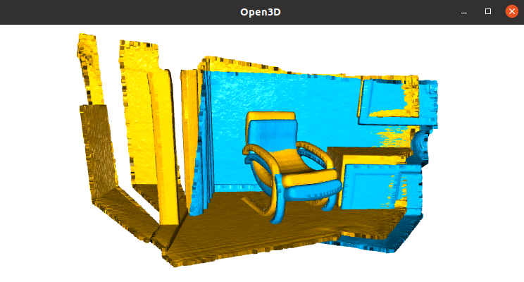
def draw_registration_result(source, target, transformation):
    # Since the functions transform() and paint_uniform_color() change the point cloud, we call copy.deepcopy to make copies and protect the original point clouds.
    source_temp = copy.deepcopy(source)
    target_temp = copy.deepcopy(target)
    source_temp.paint_uniform_color([1, 0.706, 0])
    target_temp.paint_uniform_color([0, 0.651, 0.929])
    source_temp.transform(transformation)
    o3d.visualization.draw_geometries([source_temp, target_temp],
                                      zoom=0.4459,
                                      front=[0.9288, -0.2951, -0.2242],
                                      lookat=[1.6784, 2.0612, 1.4451],
                                      up=[-0.3402, -0.9189, -0.1996])

demo_icp_pcds = o3d.data.DemoICPPointClouds()
source = o3d.io.read_point_cloud(demo_icp_pcds.paths[0])
target = o3d.io.read_point_cloud(demo_icp_pcds.paths[1])
# Initial guess transform between the two point-cloud.
# ICP algortihm requires a good initial allignment to converge efficiently.
trans_init = np.asarray([[0.862, 0.011, -0.507, 0.5],
                         [-0.139, 0.967, -0.215, 0.7],
                         [0.487, 0.255, 0.835, -1.4], [0.0, 0.0, 0.0, 1.0]])
draw_registration_result(source, target, trans_init)

Evaluation

The function evaluate_registration() calculates two main metrics:

fitness, which measures the overlapping area (# of inlier correspondences / # of points in target).
- The higher the better.
inlier_rmse, which measures the RMSE of all inlier correspondences.
- The lower the better.

 1
 2
 3
 4
 5
 6
 7
 8
 9
10
11
12


print("Initial alignment")
threshold = 0.02
evaluation = o3d.pipelines.registration.evaluate_registration(
    source, target, threshold, trans_init)
print(evaluation)
'''
RegistrationResult with
- fitness=1.747228e-01,
- inlier_rmse=1.177106e-02, and
- correspondence_set size of 34741
Access transformation to get result.
'''

Idea of ICP Algorithm

In general, the ICP algorithm iterates over two steps:

Find correspondence set $K = {(p,q)}$ from target point cloud P, and source point cloud Q transformed with current transformation matrix T
Update the transformation T by minimizing an objective function E(T) defined over the correspondence set K.

Different variants of ICP use different objective functions E(T)
- Point-to-point ICP[1]
- Point-to-plane ICP[2]
- Colored ICP[3]

2. Point-to-Point ICP

The class TransformationEstimationPointToPoint provides functions to compute the residuals and Jacobian matrices of the point-to-point ICP objective.

The function registration_icp() takes it as a parameter and runs point-to-point ICP to obtain the results.
Update the trans_init (4 x 4 matrix) by minimizing an objective function: $E(T)=\sum_{(p,q) \in K} ||p-Tq||^2$

 1
 2
 3
 4
 5
 6
 7
 8
 9
10
11
12
13
14
15
16
17
18


print("Apply point-to-point ICP")
s = time.time()
reg_p2p = o3d.pipelines.registration.registration_icp(
    source, target, threshold, trans_init,
    o3d.pipelines.registration.TransformationEstimationPointToPoint())
icp_time = time.time() - s
print("Time taken by Point-To-Plane ICP: ", icp_time) # 3.4535
print("Fitness: ", reg_p2p.fitness) # 0.372450
print("Inlier RMSE: ", reg_p2p.inlier_rmse) # 0，007760
print("Correspondence Set: ",reg_p2p.correspondence_set) # 74056
print("Transformation is:")
print(reg_p2p.transformation)
'''
[[ 0.83924644  0.01006041 -0.54390867  0.64639961]
 [-0.15102344  0.96521988 -0.21491604  0.75166079]
 [ 0.52191123  0.2616952   0.81146378 -1.50303533]
 [ 0.          0.          0.          1.        ]]
'''

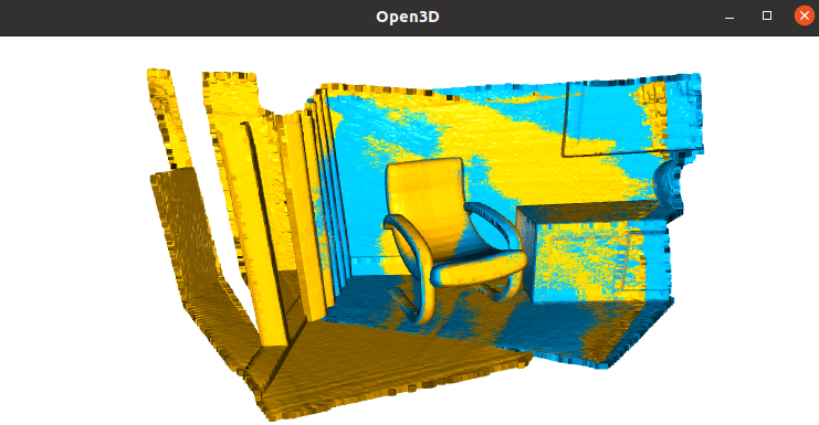
The fitness score increases from 0.174723 to 0.372450. The inlier_rmse reduces from 0.011771 to 0.007760, and correspondence_set size is 74056 from 34741

By default, registration_icp() runs until convergence or reaches a maximum number of iterations (30 by default).
It can be changed to allow more computation time and to improve the results further.
- by adding o3d.pipelines.registration.ICPConvergenceCriteria(max_iteration=2000)) as a parameter

1
2
3
4
5


reg_p2p = o3d.pipelines.registration.registration_icp(
    source, target, threshold, trans_init,
    o3d.pipelines.registration.TransformationEstimationPointToPoint(),
    o3d.pipelines.registration.ICPConvergenceCriteria(max_iteration=2000))
draw_registration_result(source, target, reg_p2p.transformation)

The final alignment is tight. The fitness score improves to 0.621123. The inlier_rmse reduces to 0.006583. The correspondence_set size improves 123501 from 74056.

3. Point-to-Plane ICP

[4] has shown that the point-to-plane ICP algorithm has a faster convergence speed than the point-to-point ICP algorithm.

by using a different objective function $E(T)=\sum_{(p,q) \in K} ((p-Tq) \times n_p)^2$
$n_p$ is the normal of point $p$
If normals are not given, they can be computed with Vertex normal estimation.

 1
 2
 3
 4
 5
 6
 7
 8
 9
10
11
12
13
14
15
16
17


print("Apply point-to-plane ICP")
reg_p2l = o3d.pipelines.registration.registration_icp(
    source, target, threshold, trans_init,
    o3d.pipelines.registration.TransformationEstimationPointToPlane())
icp_time = time.time() - s
print("Time taken by Point-To-Plane ICP: ", icp_time) # 3.4543
print("Fitness: ", reg_p2l.fitness) # 0.620972
print("Inlier RMSE: ", reg_p2l.inlier_rmse) # 0.00658
print("Correspondence Set: ",reg_p2l.correspondence_set) # 123471
print("Transformation is:")
print(reg_p2l.transformation)
'''
[[ 0.84023324  0.00618369 -0.54244126  0.64720943]
 [-0.14752342  0.96523919 -0.21724508  0.81018928]
 [ 0.52132423  0.26174429  0.81182576 -1.48366001]
 [ 0.          0.          0.          1.        ]]
'''

The point-to-plane ICP reaches tight alignment within 30 iterations

(a fitness score of 0.620972 and an inlier_rmse score of 0.006581)

4. Colored Point Cloud Registration

Colored point cloud registration uses both geometry and color for registration

The color information locks the alignment along the tangent plane.
Thus this algorithm is more accurate and more robust than prior point cloud registration algorithms,
while the running speed is comparable to that of ICP registration.

Input and Initial Transformation

An identity matrix is used as initialization for the registration.

1
2
3
4
5
6
7


demo_colored_icp_pcds = o3d.data.DemoColoredICPPointClouds()
source = o3d.io.read_point_cloud(demo_colored_icp_pcds.paths[0])
target = o3d.io.read_point_cloud(demo_colored_icp_pcds.paths[1])

# draw initial alignment
current_transformation = np.identity(4)
draw_registration_result(source, target, current_transformation)

Misaligned Point-to-Plane ICP

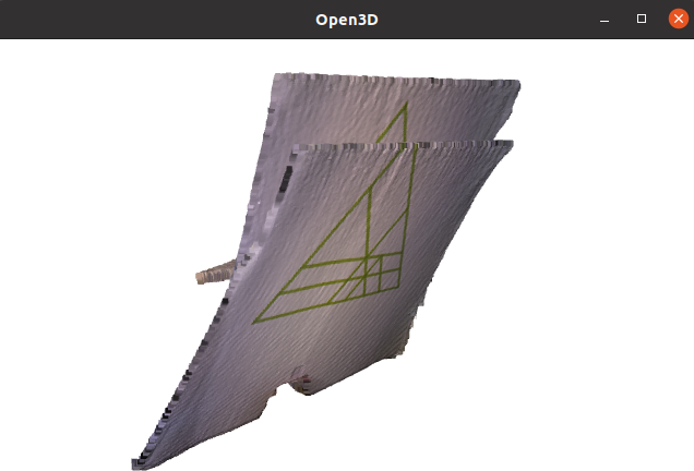
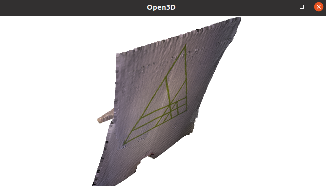
We first run Point-to-plane ICP as a baseline approach.

The visualization below shows misaligned green triangle textures.
This is because a geometric constraint does not prevent two planar surfaces from slipping.

 1
 2
 3
 4
 5
 6
 7
 8
 9
10


# point to plane ICP
current_transformation = np.identity(4)
print("2. Point-to-plane ICP registration is applied on original point")
print("   clouds to refine the alignment. Distance threshold 0.02.")
result_icp = o3d.pipelines.registration.registration_icp(
    source, target, 0.02, current_transformation,
    o3d.pipelines.registration.TransformationEstimationPointToPlane())
print(result_icp)
draw_registration_result_original_color(source, target,
                                        result_icp.transformation)

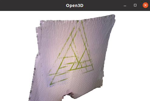
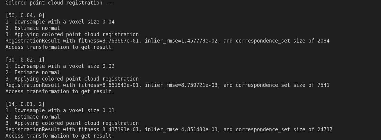
Colored ICP

To further improve efficiency, [3] proposes a multi-scale registration scheme. In total, 3 layers of multi-resolution point clouds are created with voxel_down_sample.

as voxel_down_sample decreases from 0.04 to 0.01, even less max_iter (from 50 to 14), we can still achieve better alignment (correspondence_set increases from 2084 to 24737)

 1
 2
 3
 4
 5
 6
 7
 8
 9
10
11
12
13
14
15
16
17
18
19
20
21
22
23
24
25
26
27
28
29
30
31
32
33
34


# colored pointcloud registration
# This is implementation of following paper
# J. Park, Q.-Y. Zhou, V. Koltun,
# Colored Point Cloud Registration Revisited, ICCV 2017
voxel_radius = [0.04, 0.02, 0.01]
max_iter = [50, 30, 14]
current_transformation = np.identity(4)
print("3. Colored point cloud registration")
for scale in range(3):
    iter = max_iter[scale]
    radius = voxel_radius[scale]
    print([iter, radius, scale])

    print("3-1. Downsample with a voxel size %.2f" % radius)
    source_down = source.voxel_down_sample(radius)
    target_down = target.voxel_down_sample(radius)

    print("3-2. Estimate normal.")
    source_down.estimate_normals(
        o3d.geometry.KDTreeSearchParamHybrid(radius=radius * 2, max_nn=30))
    target_down.estimate_normals(
        o3d.geometry.KDTreeSearchParamHybrid(radius=radius * 2, max_nn=30))

    print("3-3. Applying colored point cloud registration")
    result_icp = o3d.pipelines.registration.registration_colored_icp(
        source_down, target_down, radius, current_transformation,
        o3d.pipelines.registration.TransformationEstimationForColoredICP(),
        o3d.pipelines.registration.ICPConvergenceCriteria(relative_fitness=1e-6,
                                                          relative_rmse=1e-6,
                                                          max_iteration=iter))
    current_transformation = result_icp.transformation
    print(result_icp)
draw_registration_result(source, target,
                                        result_icp.transformation)

Reference

[1] Paul J. Besl and Neil D. McKay, A Method for Registration of 3D Shapes, PAMI, 1992.
[2] Y. Chen and G. G. Medioni, Object modelling by registration of multiple range images, Image and Vision Computing, 10(3), 1992.
[3] J. Park, Q.-Y. Zhou, and V. Koltun, Colored Point Cloud Registration Revisited, ICCV, 2017. [4] S. Rusinkiewicz and M. Levoy. Efficient variants of the ICP algorithm. In 3-D Digital Imaging and Modeling, 2001. [5] http://www.open3d.org/docs/release/tutorial/pipelines/icp_registration.html
[6] http://www.open3d.org/docs/release/tutorial/t_pipelines/t_icp_registration.html