Statistical Learning Notes | SVM 2 - Support Vector Classifiers and Machines

Support Vector Classifiers

2.1. Motivation

Disadvantages of Maximal Margin Classifier:

A classifier based on a separating hyperplane will necessarily perfectly classify ALL of the training observations

• this can lead to sensitivity to individual observations
  • a change in a single observation may lead to a dramatic change in the hyperplane
• it may have overfit the training data

Improvement:

Consider a classifier based on a hyperplane that does NOT perfectly separate the two classes, in the interest of:

• Greater Robustness to individual observations, and
• Better Classification of most of the training observations
  • may misclassify a few training data but may be worthwhile for trade-off

2.2. Support Vector Classifier

Rather than seeking the largest possible margin so that every observation is perfectly on the correct side,

• Support Vector Classifier (Soft Margin Classifier) instead allows some observations to be on the incorrect side
  • Soft: margin can be violated by some of the training observations

Solve Optimization Problem

M is the width of the margin,

$$\max_{\beta_0,\beta_1,\cdots,\beta_p,\ \epsilon_1,\cdots,\epsilon_n,\ M} M$$ $$s.t. \sum_{j=1}^p \beta_j^2 = 1,$$ $$y_i(\beta_0 + \sum_{k=1}^p\beta_kx_{ik})\geq M(1-\epsilon_i),$$ $$\epsilon_i \geq 0, \ \sum_{i=1}^n\epsilon_i \leq C,$$

Parameters:

$\epsilon_i$ is slack variable that allows individual observation to be on the wrong side of the margin or the hyperplane

• it tells us where the ith observation is located, relative to the hyperplane and relative to the margin
  • if $\epsilon_i=0$ then the ith observation is on the correct side of the margin
  • if $\epsilon_i>0$ then the ith observation is on the wrong side of the margin
  • if $\epsilon_i>1$ then the ith observation is on the wrong side of the hyperplane

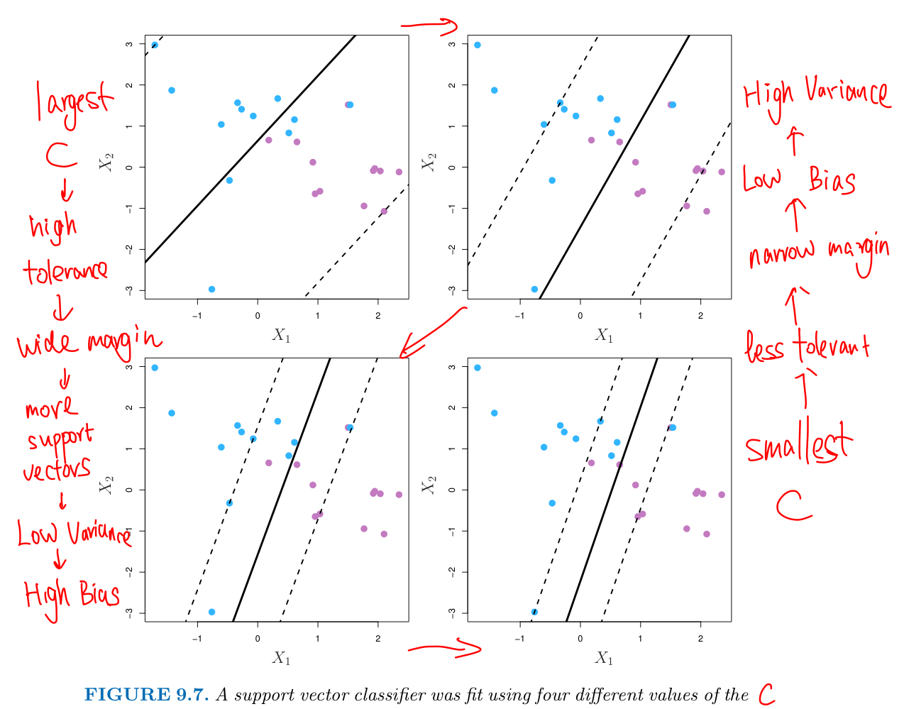
C is a nonnegative tuning (or regularization) parameter that is chosen via Cross-Validation

• C bounds the sum of the $\epsilon_i$ ,
• and so it determines the number of severity of the violations to the margin (and hyperplane)
  • C is considered as a Budget for the amount that the margin can be violated by the n observations
  • if C = 0, NO Budget for violations to the margin, all $\epsilon_i = 0$
  • if C > 0, no more than C observations can be on the wrong side of the hyperplane
    • since $\epsilon_i>1$ and $\sum_{i=1}^n\epsilon_i \leq C$
  • As C increases, more tolerant of violations to the margin
    • the margin will widen so fit the data less hard
    • Low Variance but More Bias
      • since many observations are support vectors that determine the hyperplane
  • As C decreases, the margin narrows so is rarely violated
    • this amounts to a classifiers that is highly fit to the data
    • Low Bias but High Variance
      • fewer support vectors

Property：

ONLY observations that either lie on the margin or violate the margin will affect hyperplane and hence the classifier obtained.

• those observations are known as Support Vectors and do affect Support Vector Classifier
• an observation that lies strictly on the correct side of the margin does NOT affect the Support Vector Classifier

SVC’s decision rule is based ONLY on the support vectors (a small subset of the training observations）

• it is quite Robust to the behavior of observations that are far away from the hyperplane
• vs LDA （different): classification rule depends on the mean of ALL of the observations within each class
  • as well as the within-class covariance matrix computed using ALL of the observations
• vs Logistic（closely related): low sensitivity to observations far from the decision boundary.
• A detailed comparison of Classification Methods will be seen in next note！

2.3. Support Vector Machines

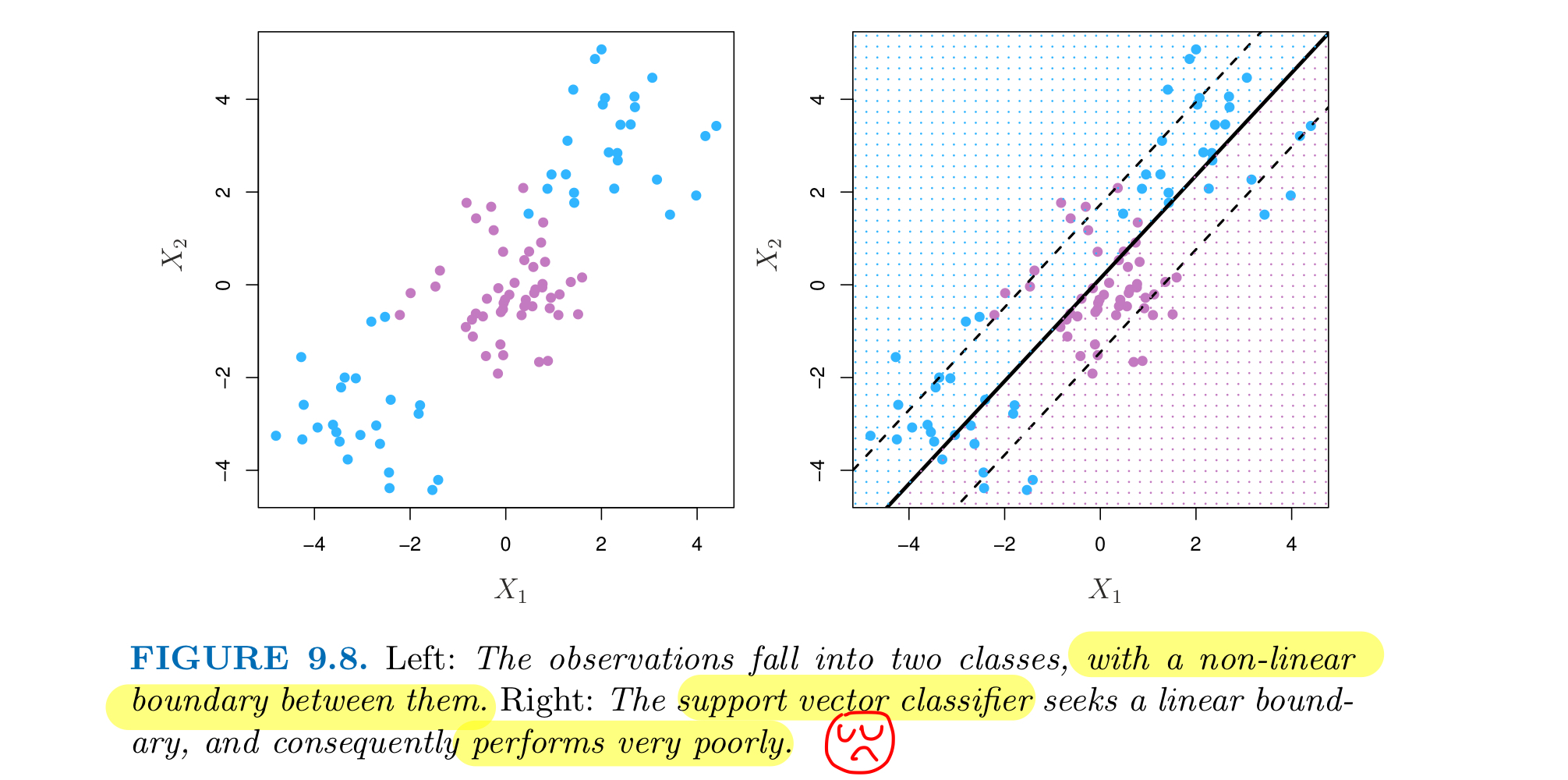
Classification with Non-Linear Decision Boundaries

Support Vector Classifiers are useless if the boundary between the two classes is Non-Linear.

TO address non-linear boundaries problem, we could enlarging the feature space using quadratic, cubic and even higher-order polynomial functions of the predictors

• rather than fitting a SVC using p features: $X_1,X_2,\cdots,X_p$
• we could instead fit a SVC using 2p features: $$X_1,X_1^2,X_2,X_2^2\cdots,X_p,X_p^2$$

Solve Optimization Problem

$$\max_{\beta_0,\beta_{11},\beta_{12}, \cdots,\beta_{p1}, \beta_{p2}, \ \epsilon_1,\cdots,\epsilon_n,\ M} M$$ $$s.t. \ y_i(\beta_0 + \sum_{j=1}^p\beta_{j1}x_{ij} + \sum_{j=1}^p\beta_{j2}x_{ij}^2)\geq M(1-\epsilon_i),$$ $$\epsilon_i \geq 0, \ \sum_{i=1}^n\epsilon_i \leq C, \sum_{j=1}^p \sum_{k=1}^2 \beta_{jk}^2 = 1,$$

This leads to a non-linear decision boundary because:

• In the enlarged feature space, the decision boundary is in fact Linear
• In the original feature space, the decision boundary is of the form q(x) = 0, where q is a quadratic polynomial
  • and its solutions a generally Non-Linear
• Con: polynomials are wild but inefficient to enlarge feature space
  • unmanageable computations

Using Kernels to Enlarge Feature Space

A kernel is a function that quantifies the similarity of two observations

• more elegant and controlled way to introduce nonlinearities and efficient computations in SVC

Linear Kernel:
$$K(x_i,x_{i'}) = \sum_{j=1}^p x_{ij}x_{i’j} = <x_i, x_{i'}> - - \text{inner product between two vectors}$$

• The Linear Kernel quantifies the similarity of a pair of observations using Pearson(standard) Correlation

The Linear SVC can be represented as $$f(x) = \beta_0 + \sum^n_{i=1}\alpha_i <x,x_i> - - \text{n parameters}$$

• To Estimate the Parameters $\beta_0, \alpha_0, \cdots, \alpha_n$, we need ALL
  • $\binom{n}{2}$ inner products $<x_i, x_{i'}>$ between ALL pairs of n training observations
• Solution: $\alpha_i > 0$ ONLY for the Support Vectors
  • and the other $\alpha_i = 0$ if a training observation is NOT a support vector
• Summary: to represent the linear classifier f(x), and to compute its coefficient - all we need are inner products

Polynomial Kernel:
$$K(x_i,x_{i'}) = (1 + \sum_{j=1}^p x_{ij}x_{i’j})^d$$

• using such a kernel with degree d > 1 leads to a MUCH MORE flexible decision boundary
• when SVC is combined with a Non-Linear Kernel,
  • the resulting classifier is known as Support Vector Machine

To compute the inner-products needed for d dimensional polynomials

• $\binom{p+d}{d}$ basis functions, we get the non-linear function with the form: $$f(x) = \beta_0 + \sum_{i \in S}\alpha_i K(x,x_i)$$
• S is the collection of indices of Support Vectors

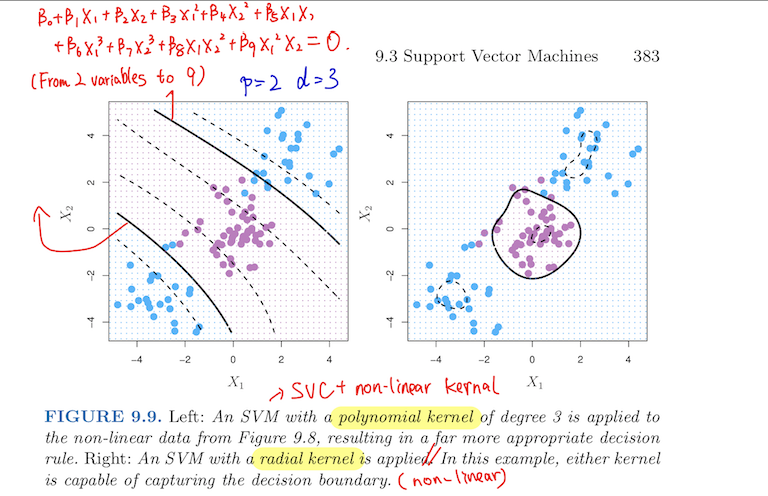
Radial Kernel
$$K(x_i,x_{i'}) = exp(-\gamma \sum_{j=1}^p(x_{ij}-x_{i’j})^2)$$

• part of Multivariate Gaussian Distribution
• the feature space is infinite-dimensional and implicit
  • because Taylor Series Expansion for $e^{x_1,x_2}$ can be represented by infinite inner product
  • when fitting the data, many of the dimensions are squashed down heavily
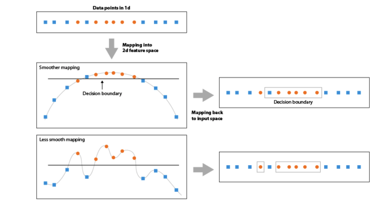
• smaller $\gamma$ => lower variance, higher biase=> smoother(simpler) decision boundaries
  • because Larger RBF kernel bandwidths produce smoother feature space mappings
• larger $\gamma$ => higher variance => more flexible(complex) decision boundaries (less smooth)
  • fit becomes more non-linear
  • lower training error rates but higher testing error rates - overfit!

    

If a given test observation $x = (x_1,\ldots,x_p)^T$ is far from a training observation $x_i$ in terms of Euclidean Distance,

• then $\sum_{j=1}^p(x_j-x_{ij})^2$ will be _large_
• and so $K(x,x_{i}) = exp(-\gamma \sum_{j=1}^p(x_j-x_{ij})^2)$ will be _tiny_
• recall that the predicted class label for the test observation $x$ is based on the sign of f(x)
  • far training observations do not have an effect on the test observation x

Radial Kernel has very Local Behavior, ONLY Nearby training observations have an effect on how we classify a new test observation

Advantage of Kernels

Efficient Computations ONLY compute $K(x_i,x_{i'})$ for all n(n-1)/2 distinct pairs $x_i, x_i'$.

• this can be done WITHOUT explicitly working in the enlarged feature space, which may be so large that computations are intractable