Open3D Notes 01 | Point Cloud Processing

2022-07-04 990 words 5 minutes

Contents

0. Download and Install Open3D

1
2
3
4
5
6
7
8


# Install
$ pip install open3d

# Verify
$ python -c "import open3d as o3d; print(o3d.__version__)"
# 0.15.2 (2022.06.28)
# Git Clone
$ git clone https://github.com/isl-org/Open3D.git

1. Read and Write a Point Cloud.

 1
 2
 3
 4
 5
 6
 7
 8
 9
10


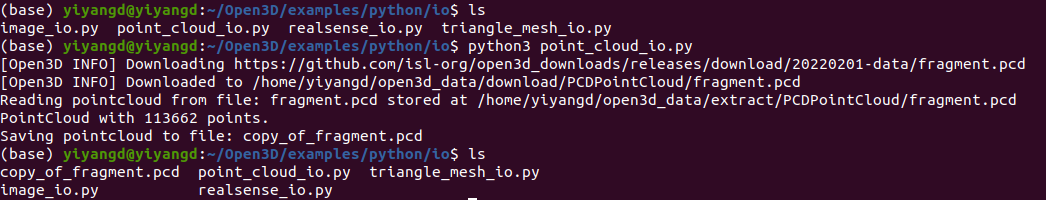
import open3d as o3d

if __name__ == "__main__":
    pcd_data = o3d.data.PCDPointCloud()
    print(
        f"Reading pointcloud from file: fragment.pcd stored at {pcd_data.path}")
    pcd = o3d.io.read_point_cloud(pcd_data.path)
    print(pcd)
    print("Saving pointcloud to file: copy_of_fragment.pcd")
    o3d.io.write_point_cloud("copy_of_fragment.pcd", pcd)

Check the folder before and after o3d.io.write_point_cloud()

2. Visualize Point Cloud

1
2
3
4
5
6
7
8
9



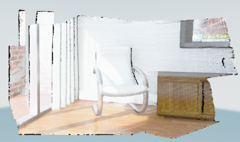
print("Load a ply point cloud, print it, and render it")
sample_ply_data = o3d.data.PLYPointCloud()
pcd = o3d.io.read_point_cloud(sample_ply_data.path)
# Flip it, otherwise the pointcloud will be upside down.
pcd.transform([[1, 0, 0, 0], [0, -1, 0, 0], [0, 0, -1, 0], [0, 0, 0, 1]])
print(pcd)
# PointCloud with 196133 points.
o3d.visualization.draw_geometries([pcd])

It looks like a dense surface, but it is actually a point cloud rendered as surfels.

The GUI supports various keyboard functions.
For instance, the - key reduces the size of the points (surfels).

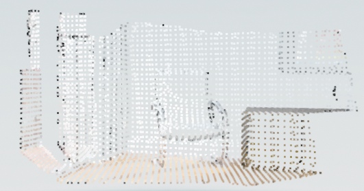
3. Voxel Downsampling

Voxel downsampling uses a regular voxel grid to create a uniformly downsampled point cloud from an input point cloud.

Voxel in 3D point cloud = Pixel in 2D image
It is often used as a pre-processing step for many point cloud processing tasks.

The algorithm operates in two steps:

Points are bucketed into voxels.
Each occupied voxel generates exactly one point by averaging all points inside.

1
2
3
4


print("Downsample the point cloud with a voxel of 0.05")
downpcd = pcd.voxel_down_sample(voxel_size=0.05)
print(downpcd) # PointCloud with 4838 points.
o3d.visualization.draw_geometries([downpcd])

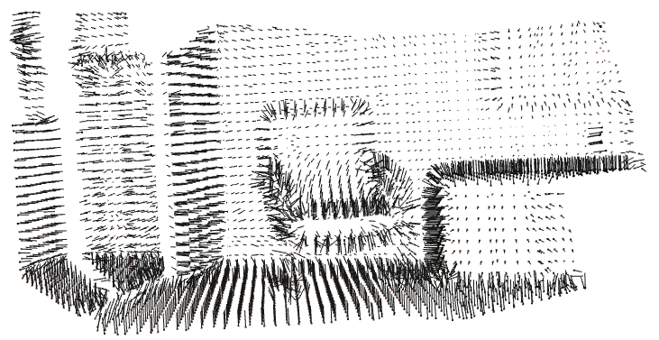
4. Vertex Normal Estimation

estimate_normals() computes the normal for every point.

The function finds adjacent points and calculates the principal axis of the adjacent points using covariance analysis.
The function takes an instance of KDTreeSearchParamHybrid class as an argument.
- it specifies search radius radius = 0.1 and maximum nearest neighbor max_nn=30 to save computation time.

1
2
3
4
5


print("Recompute the normal of the downsampled point cloud")
downpcd.estimate_normals(
    search_param=o3d.geometry.KDTreeSearchParamHybrid(
    radius=0.1, max_nn=30))
o3d.visualization.draw_geometries([downpcd],point_show_normal=True)

Open3D tries to orient the normal to align with the original normal if it exists.

Otherwise, Open3D does a random guess.
Further orientation functions such as orient_normals_to_align_with_direction and orient_normals_towards_camera_location need to be called if the orientation is a concern.

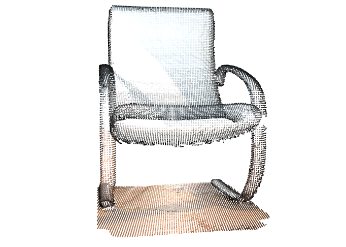
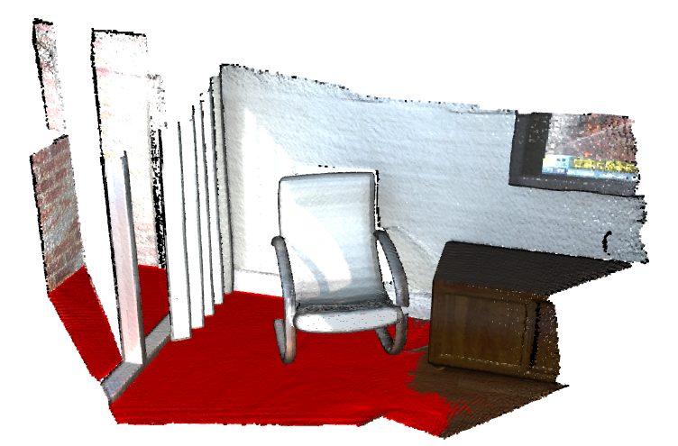
5. Crop Point Cloud

read_selection_polygon_volume() reads a json file that specifies polygon selection area.
vol.crop_point_cloud(pcd) filters out points. Only the chair remains.

 1
 2
 3
 4
 5
 6
 7
 8
 9
10
11
12
13
14


  print("Load a ply point cloud, crop it, and render it")
  sample_ply_data = o3d.data.DemoCropPointCloud()
  pcd = o3d.io.read_point_cloud(sample_ply_data.point_cloud_path)
  vol = o3d.visualization.read_selection_polygon_volume(
      sample_ply_data.cropped_json_path)
  chair = vol.crop_point_cloud(pcd)
  # Flip the pointclouds, otherwise they will be upside down.
  pcd.transform([[1, 0, 0, 0], [0, -1, 0, 0], [0, 0, -1, 0], [0, 0, 0, 1]])
  chair.transform([[1, 0, 0, 0], [0, -1, 0, 0], [0, 0, -1, 0], [0, 0, 0, 1]])

  print("Displaying original pointcloud ...")
  o3d.visualization.draw([pcd])
  print("Displaying cropped pointcloud")
  o3d.visualization.draw([chair])

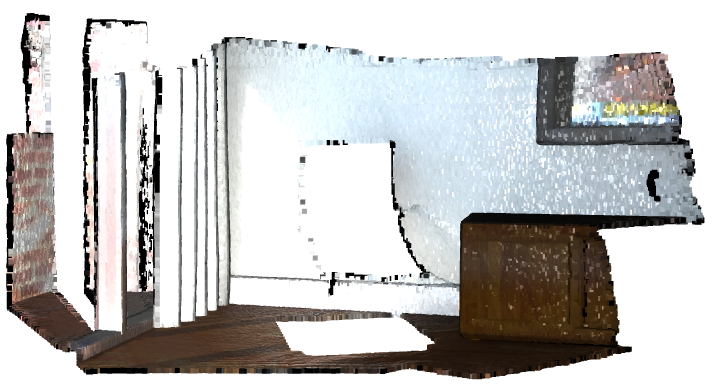
6. Paint Point Cloud

paint_uniform_color([R,G,B]) paints all the points to a uniform color.

The color is in RGB space, [0, 1] range.

1
2
3


print("Paint chair")
chair.paint_uniform_color([1, 0.706, 0])
o3d.visualization.draw_geometries([chair])

7. Point Cloud Distance

source.compute_point_cloud_distance(target) computes for each point in the source point cloud the distance to the closest point in the target point cloud.

1
2
3
4
5
6
7
8
9



dists = pcd.compute_point_cloud_distance(chair)
dists = np.asarray(dists)
print("Printing average distance between the two point clouds ...")
print(dists) # .shape = # of points
# Filter out the points that has distance from the chair
ind = np.where(dists > 0.01)[0]
pcd_without_chair = pcd.select_by_index(ind)
o3d.visualization.draw_geometries([pcd_without_chair])

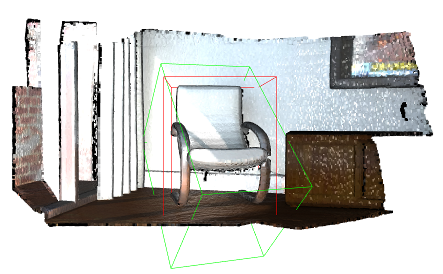
8. Bounding Volumes

Open3D implements an AxisAlignedBoundingBox and an OrientedBoundingBox that can also be used to crop the geometry.

 1
 2
 3
 4
 5
 6
 7
 8
 9
10



axis_aligned = pcd.get_axis_aligned_bounding_box()
axis_aligned.color = (1, 0, 0)
oriented = pcd.get_oriented_bounding_box()
oriented.color = (0, 1, 0)
print(
    "Displaying axis_aligned_bounding_box in red and oriented bounding box in green ..."
)
o3d.visualization.draw(
    [pcd, axis_aligned, oriented])

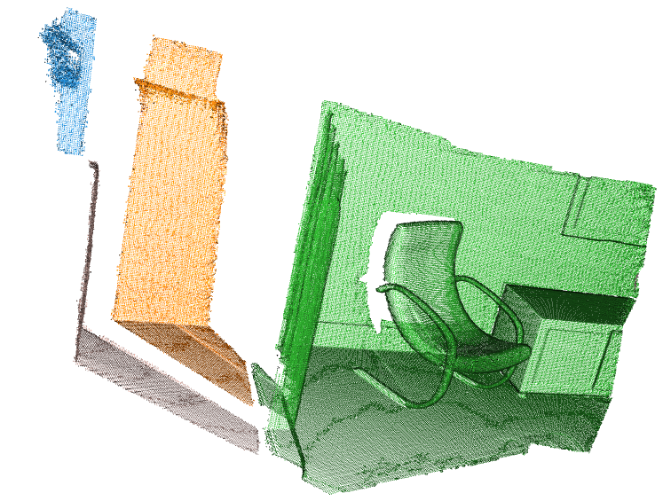
9. DBSCAN Clustering

Given a Point Cloud from a RGB-Depth sensor, we want to group local point cloud clusters together.

Open3D implements DBSCAN [Ester1996] that is a Density-based clustering algorithm.
The algorithm is implemented in cluster_dbscan and requires two parameters:
- eps defines the distance to neighbors in a cluster and
- min_points defines the minimum number of points required to form a cluster.
The function returns labels, where the label -1 indicates noise.

 1
 2
 3
 4
 5
 6
 7
 8
 9
10
11
12
13
14
15


ply_point_cloud = o3d.data.PLYPointCloud()
pcd = o3d.io.read_point_cloud(ply_point_cloud.path)

with o3d.utility.VerbosityContextManager(
        o3d.utility.VerbosityLevel.Debug) as cm:
    labels = np.array(
        pcd.cluster_dbscan(eps=0.02, min_points=10, print_progress=True))

max_label = labels.max()
print(f"point cloud has {max_label + 1} clusters")
# max_label + 1 = 10 clusters
colors = plt.get_cmap("tab20")(labels / (max_label if max_label > 0 else 1))
colors[labels < 0] = 0
pcd.colors = o3d.utility.Vector3dVector(colors[:, :3])
o3d.visualization.draw_geometries([pcd]])

10. Plane Segmentation

Open3D also supports segmententation of geometric primitives from point clouds using RANSAC.

To find the plane with the largest support in the point cloud, we can use segment_plane() with its three arguments:
- distance_threshold defines the maximum distance a point can have to an estimated plane to be considered an inlier
- ransac_n defines the number of points that are randomly sampled to estimate a plane
- num_iterations defines how often a random plane is sampled and verified.

 1
 2
 3
 4
 5
 6
 7
 8
 9
10
11
12


plane_model, inliers = pcd.segment_plane(
        distance_threshold=0.01,
        ransac_n=3,
        num_iterations=1000)
[a, b, c, d] = plane_model
print(f"Plane equation: {a:.2f}x + {b:.2f}y + {c:.2f}z + {d:.2f} = 0")
# 0x+1y+0.02z+2.43=0
print("Displaying pointcloud with planar points in red ...")
inlier_cloud = pcd.select_by_index(inliers)
inlier_cloud.paint_uniform_color([1.0, 0, 0])
outlier_cloud = pcd.select_by_index(inliers, invert=True)
o3d.visualization.draw_geometries([inlier_cloud, outlier_cloud])

The function then returns the plane as (a,b,c,d) such that for each point (x,y,z) on the plane we have ax+by+cz+d=0.

The function further returns a list of indices of the inlier points.

Reference

[1] http://www.open3d.org/docs/latest/
[2] https://github.com/isl-org/Open3D
[3] http://www.open3d.org/docs/release/tutorial/geometry/file_io.html
[4] http://www.open3d.org/docs/release/tutorial/geometry/pointcloud.html