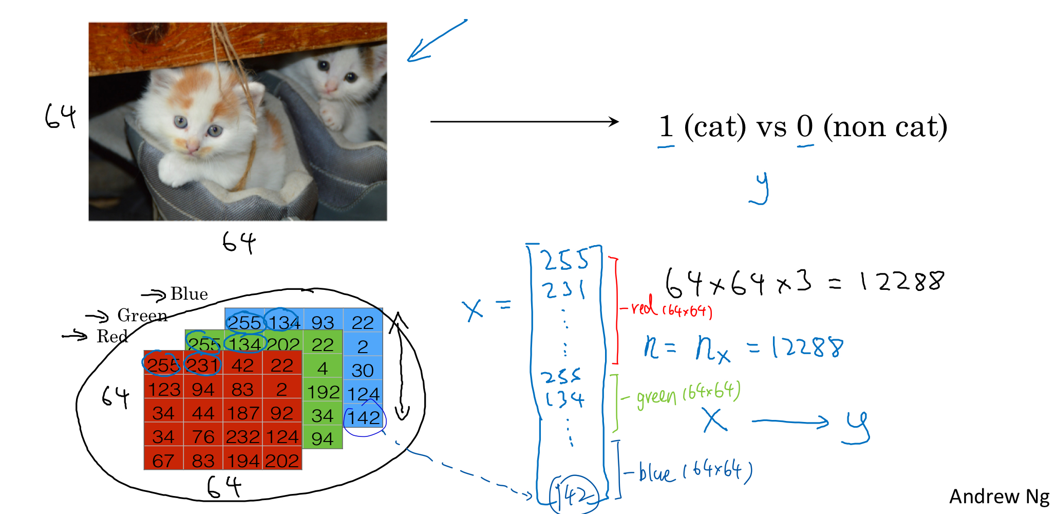
Recall: Logistic Regression is an Algorithm for Binary Classification
An image is store in the computer in three separate matrices
corresponding to the Red, Green, and Blue color channels of the image.
The three matrices have the same size as the image, for example, the resolution of the cat image is (64 pixels X 64 pixels), the three matrices (RGB) are 64 X 64 each.
 1
 2
 3
 4
 5
 6
 7
 8
 9
10
11
12
13
importnumpyasnpdefimage2vector(image):"""
Argument:
image -- a numpy array of shape (length, height, depth)
Returns:
vector -- a vector of shape (length*height*depth, 1)
"""vector=image.reshape(image.shape[0]*image.shape[1]*image.shape[2],1)returnvector
2. Sigmoid Function for LR
Given $X \in \R^{n_x}$, we want $\hat{y} = P(y=1|x), \hat{y} \in [0,1]$
Parameters: $w \in \R^{n_x}, b \in \R$
Let $z = w^T x + b$
Output:
$$\hat{y} = \sigma (z) = \frac{1}{1+e^z}$$
if z positive infinity: $\sigma (z) \approx \frac{1}{1+0} = 1$
if z negative infinity: $\sigma (z) \approx \frac{1}{1+\infty} = 0 $
 1
 2
 3
 4
 5
 6
 7
 8
 9
10
11
12
defsigmoid(z):"""
Compute the sigmoid of z
Arguments:
z -- A scalar or numpy array of any size.
Return:
s -- sigmoid(z)
"""s=1/(1+np.exp(-z))returns
3. Cost Function for Logistic Regression
Given m training data: {$(x^{(1)},y^{(1)}), \dots, (x^{(m)},y^{(m)})$}
Loss Function
$$L(\hat{y}, y) = - (y \log(\hat{y}) + (1-y) \log(1-\hat{y}))$$
if $y = 1$, $L(\hat{y}, y) = - \log(\hat{y})$, to make L as small as possible, let $\hat{y} \approx 1$
if $y = 0$, $L(\hat{y}, y) = - \log(1-\hat{y})$, to make L as small as possible, let $\hat{y} \approx 0$
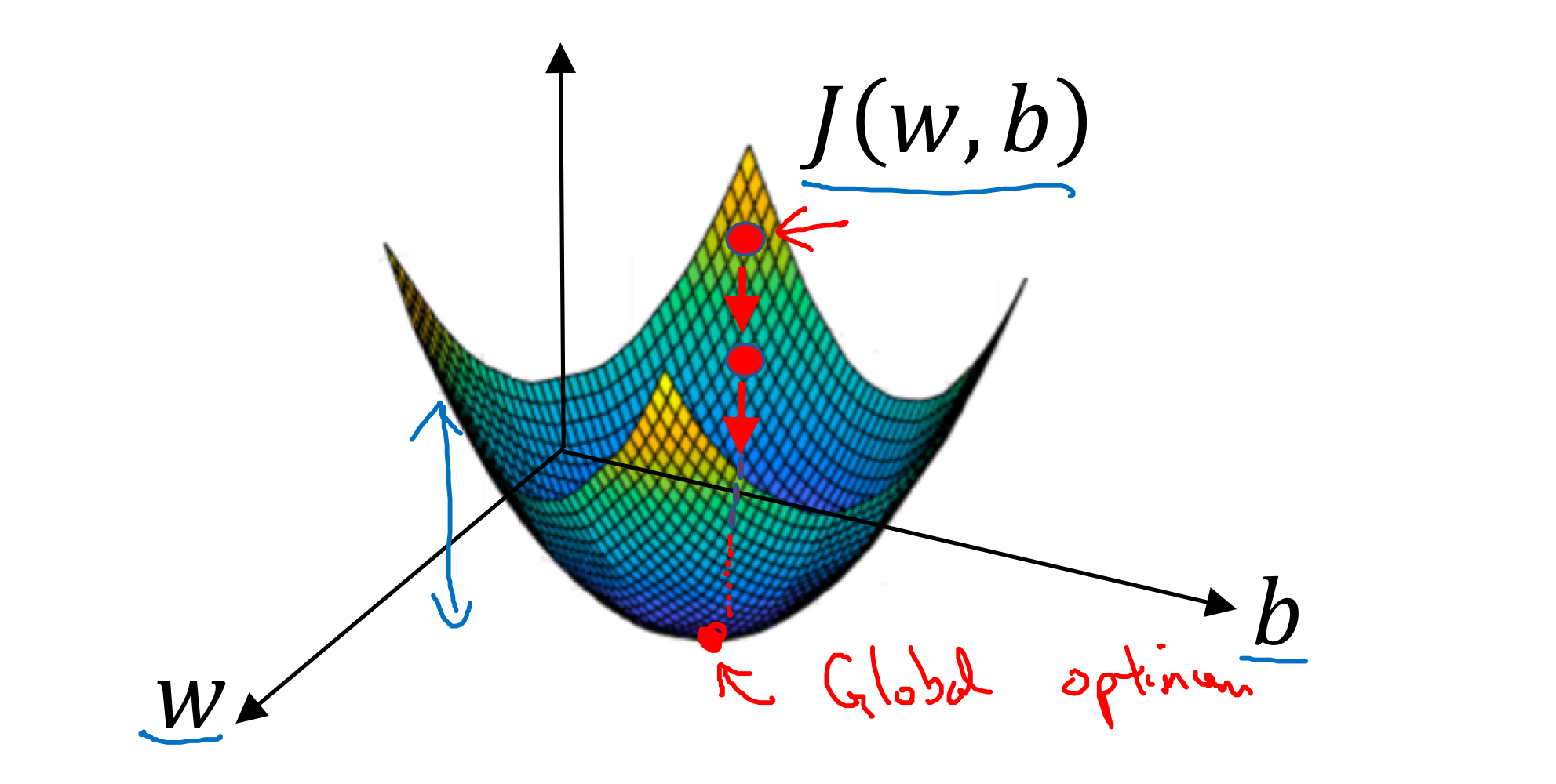
Cost Function
Goal: Use Gradient Descent to optimize the _parameters w and b* to minimize the Cost Function:
$$J(w,b)=\frac{1}{m}\sum^m_{i=1} L(\hat{y}^{(i)}, y^{(i)})$$
$$= - \frac{1}{m}\sum^m_{i=1} [y^{(i)}\log (\hat{y}^{(i)}) - (1-y^{(i)})\log (1-\hat{y}^{(i)})]$$
the cost function is a Convex Function that has a Global (Minimum) Optimum point
4. Gradient Descent
Start at the Initial Point (w, b) and take a step in the steepest downhill direction
definitialize_with_zeros(dim):"""
This function creates a vector of zeros of shape (dim, 1) for w and initializes b to 0.
Argument:
dim -- size of the w vector we want (or number of parameters in this case)
Returns:
w -- initialized vector of shape (dim, 1)
b -- initialized scalar (corresponds to the bias)
"""w=np.zeros((dim,1))b=0assert(w.shape==(dim,1))assert(isinstance(b,float)orisinstance(b,int))returnw,bdim=2w,b=initialize_with_zeros(dim)print("w = "+str(w))print("b = "+str(b))'''
w = [[0.]
[0.]]
b = 0
'''
defpropagate(w,b,X,Y):"""
Implement the cost function and its gradient for the propagation explained above
Arguments:
w -- weights, a numpy array of size (num_px * num_px * 3, 1)
b -- bias, a scalar
X -- data of size (num_px * num_px * 3, number of examples)
Y -- true "label" vector (containing 0 if non-cat, 1 if cat) of size (1, number of examples)
Return:
cost -- negative log-likelihood cost for logistic regression
dw -- gradient of the loss with respect to w, thus same shape as w
db -- gradient of the loss with respect to b, thus same shape as b
"""m=X.shape[1]# FORWARD PROPAGATION (FROM X TO COST)A=sigmoid(np.dot(w.T,X)+b)# compute activationcost=np.sum(((-np.log(A))*Y+(-np.log(1-A))*(1-Y)))/m# compute cost# BACKWARD PROPAGATION (TO FIND GRAD)dw=(np.dot(X,(A-Y).T))/mdb=(np.sum(A-Y))/massert(dw.shape==w.shape)assert(db.dtype==float)cost=np.squeeze(cost)assert(cost.shape==())grads={"dw":dw,"db":db}returngrads,cost
5. Optimization
Write down the optimization function. The goal is to learn $w$ and $b$ by minimizing the cost function $J$. For a parameter $\theta$, the update rule is $\theta = \theta - \alpha \text{ } d\theta$, where $\alpha$ is the learning rate.
defoptimize(w,b,X,Y,num_iterations,learning_rate,print_cost=False):"""
This function optimizes w and b by running a gradient descent algorithm
Arguments:
w -- weights, a numpy array of size (num_px * num_px * 3, 1)
b -- bias, a scalar
X -- data of shape (num_px * num_px * 3, number of examples)
Y -- true "label" vector (containing 0 if non-cat, 1 if cat), of shape (1, number of examples)
num_iterations -- number of iterations of the optimization loop
learning_rate -- learning rate of the gradient descent update rule
print_cost -- True to print the loss every 100 steps
Returns:
params -- dictionary containing the weights w and bias b
grads -- dictionary containing the gradients of the weights and bias with respect to the cost function
costs -- list of all the costs computed during the optimization, this will be used to plot the learning curve.
Tips:
You basically need to write down two steps and iterate through them:
1) Calculate the cost and the gradient for the current parameters. Use propagate().
2) Update the parameters using gradient descent rule for w and b.
"""costs=[]foriinrange(num_iterations):# Cost and gradient calculationgrads,cost=propagate(w,b,X,Y)# Retrieve derivatives from gradsdw=grads["dw"]db=grads["db"]# update rulew=w-(learning_rate*dw)b=b-(learning_rate*db)# Record the costsifi%100==0:costs.append(cost)# Print the cost every 100 training iterationsifprint_costandi%100==0:print("Cost after iteration %i: %f"%(i,cost))params={"w":w,"b":b}grads={"dw":dw,"db":db}returnparams,grads,costs
defpredict(w,b,X):'''
Predict whether the label is 0 or 1 using learned logistic regression parameters (w, b)
Arguments:
w -- weights, a numpy array of size (num_px * num_px * 3, 1)
b -- bias, a scalar
X -- data of size (num_px * num_px * 3, number of examples)
Returns:
Y_prediction -- a numpy array (vector) containing all predictions (0/1) for the examples in X
'''m=X.shape[1]Y_prediction=np.zeros((1,m))w=w.reshape(X.shape[0],1)# Compute vector "A" predicting the probabilities of a cat being present in the pictureA=sigmoid(np.dot(w.T,X)+b)# Dimentions = (1, m)Y_prediction=(A>=0.5)*1.0# 1 if A >= 0.5, 0 otherwiseassert(Y_prediction.shape==(1,m))returnY_prediction
defmodel(X_train,Y_train,X_test,Y_test,num_iterations=2000,learning_rate=0.5,print_cost=False):"""
Builds the logistic regression model by calling the function you've implemented previously
Arguments:
X_train -- training set represented by a numpy array of shape (num_px * num_px * 3, m_train)
Y_train -- training labels represented by a numpy array (vector) of shape (1, m_train)
X_test -- test set represented by a numpy array of shape (num_px * num_px * 3, m_test)
Y_test -- test labels represented by a numpy array (vector) of shape (1, m_test)
num_iterations -- hyperparameter representing the number of iterations to optimize the parameters
learning_rate -- hyperparameter representing the learning rate used in the update rule of optimize()
print_cost -- Set to true to print the cost every 100 iterations
Returns:
d -- dictionary containing information about the model.
"""# initialize parameters with zeros (≈ 1 line of code)w,b=initialize_with_zeros(X_train.shape[0])# Gradient descent (≈ 1 line of code)parameters,grads,costs=optimize(w,b,X_train,Y_train,num_iterations,learning_rate,print_cost)# Retrieve parameters w and b from dictionary "parameters"w=parameters["w"]b=parameters["b"]# Predict test/train set examplesY_prediction_test=predict(w,b,X_test)Y_prediction_train=predict(w,b,X_train)# Print train/test Errorsprint("train accuracy: {} %".format(100-np.mean(np.abs(Y_prediction_train-Y_train))*100))print("test accuracy: {} %".format(100-np.mean(np.abs(Y_prediction_test-Y_test))*100))d={"costs":costs,"Y_prediction_test":Y_prediction_test,"Y_prediction_train":Y_prediction_train,"w":w,"b":b,"learning_rate":learning_rate,"num_iterations":num_iterations}returnd