Time Series Note | Financial Time Series Analysis

1. Introduction to Time Series in Python

Time Series is a sequence of information which attaches a time period to each value

• A common topic in Time Series Analysis is determining the stability of financial markets and the efficiency protfolios (效率投资组合)

Properties

All time-periods must be equal and clearly defined, which would result in a constant frequency

• Frequency: how often values of the data set are recorded
• if the intervals are not identical => dealing with missing data

Time-Dependency(时效性): the values for every period are affected by outside factors and by the values of past periods

• in chronological order
• from a machine learning perspective, this is inconvenient for train/test data split
  • we need pick a cut-off point and let the period before the cut-off point be the training set and the period after the cutoff point be the testing set

Python Implementation

Step1: Import the library and read the file

• Create a copy of original data in case we erase certain values and read the csv file again
• df.head() shows the information of the top five observations for the data set

1
2
3
4
5
6
7

import pandas as pd
import numpy as np

raw_csv_data = pd.read_csv("Index2018.csv")
df_comp = raw_csv_data.copy()

df_comp.head()

Output:

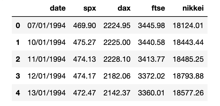
• date: represents the day when the values of the other columns (closing prices of four market indexes) were recorded
• Each market index is a portfolio of the most traded companies on the respective stock exchange markets:
• spx: S&P 500 measures the stability of the US stock exchanges
• dax: DAX 30 measures the stability of the German stock exchanges
• ftse: FTSE 100 measures the stability of the London Stock exchanges
• nikkei: NIKKEI 225 measures the stability of the Japanese stock exchanges

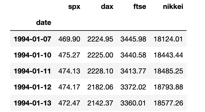
Step2: Transform “dd/mm/yyyy” format to “yyyy-mm-dd” datetime format

• set date as index: inplace = True lets date replace the integer index
  • Once “date” becomes an index, we no longer save/modify its values as a seperate attribute in the data frame
• set frequency:
  • arguments: ‘h’ - hourly, ‘w’ - weekly, ’d' - daily, ’m' - monthly
  • not interested in any weekends or holidays => missing values NaN
  • ‘b’ - business days

1
2
3
4

df_comp.date = pd.to_datetime(df_comp.date, dayfirst = True)
df_comp.set_index("date", inplace = True)
df_comp = df_comp.asfreq('b')
df_comp.head()

Output:

Step3: Handling Missing Values

• For each attribute, df_comp.isna().sum() will show the number of instances without available information for each column
• Setting the frequency to “business days” must have generated 8 dates, for which we have no data available
• fillna() method:
  • front filling: assigns the value of the previous period
  • back filling: assigns the value for the next period
  • assigning the same average to all the missing values (bad approach)

1
2
3
4
5

df_comp.spx = df_comp.spx.fillna(method = "ffill")
df_comp.ftse = df_comp.ftse.fillna(method = "bfill")
df_comp.dax = df_comp.dax.fillna(value = df_comp.dax.mean())
# to count the missing values
df_comp.isna().sum()

Step4: Adding and Removing Columns

• just keep the index time and spx as market_value

1
2

df_comp['market_value'] = df_comp.spx
del df_comp['spx'], df_comp['dax'], df_comp['ftse'], df_comp['nikkei']

Step5: Splitting the Time-Series data

• since time series data relies on keeping the chronological order of the values
  • cannot “shuffle” the data before splitting
• Training Set: From the beginning up to some cut off point
• Testing Set: From the cut off point until the end
• 80-20 split is resonable
  • training set too large: performs poorly with new data
  • training set too small: cannot create an accurate model
• iloc comes from index location
• len comes from length
• int ensures that the train_size will be integer

1
2
3
4
5

train_size = int(len(df_comp)*0.8)
df_train, df_test = df_comp.iloc[:train_size], df_comp.iloc[train_size:]
# check if there is overlapping data
df_train.tail()
df_test.head()

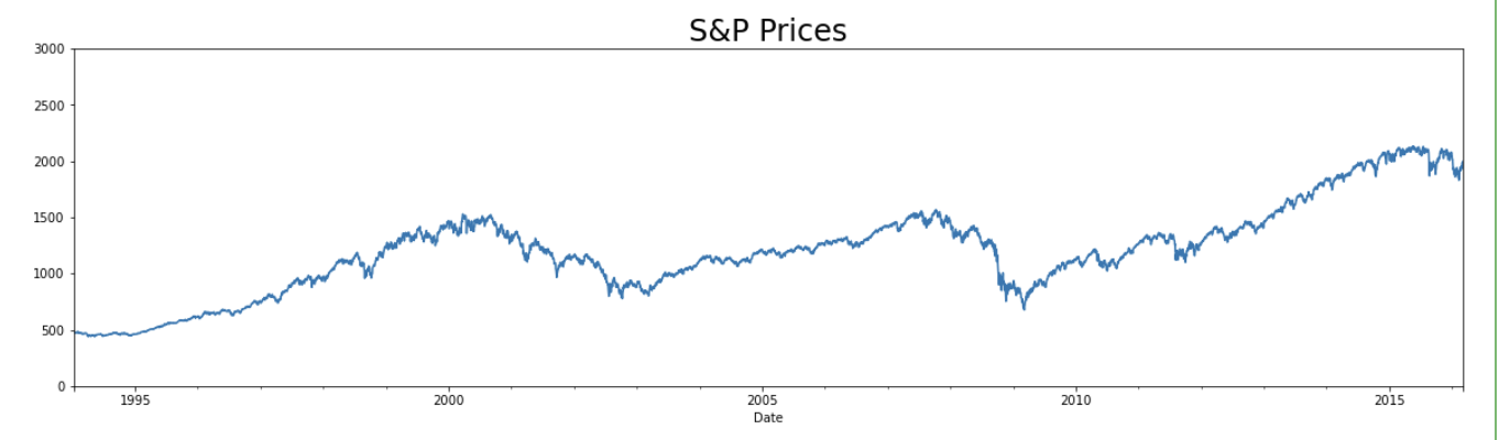
Step6: Data Visualization

1
2
3
4
5

import matplotlib.pyplot as plt
df_train.market_value.plot(figsize = (20,5))
plt.title("S&P Prices", size=24)
plt.ylim(0,3000)
plt.show()

Output:

The QQ Plot is a tool used to determine whether a data set is distributed a certain way (normal)

1
2
3
4

import scipy.stats
import pylab
scipy.stats.probplot(df_comp.spx, plot = pylab)
pylab.show()

Output:

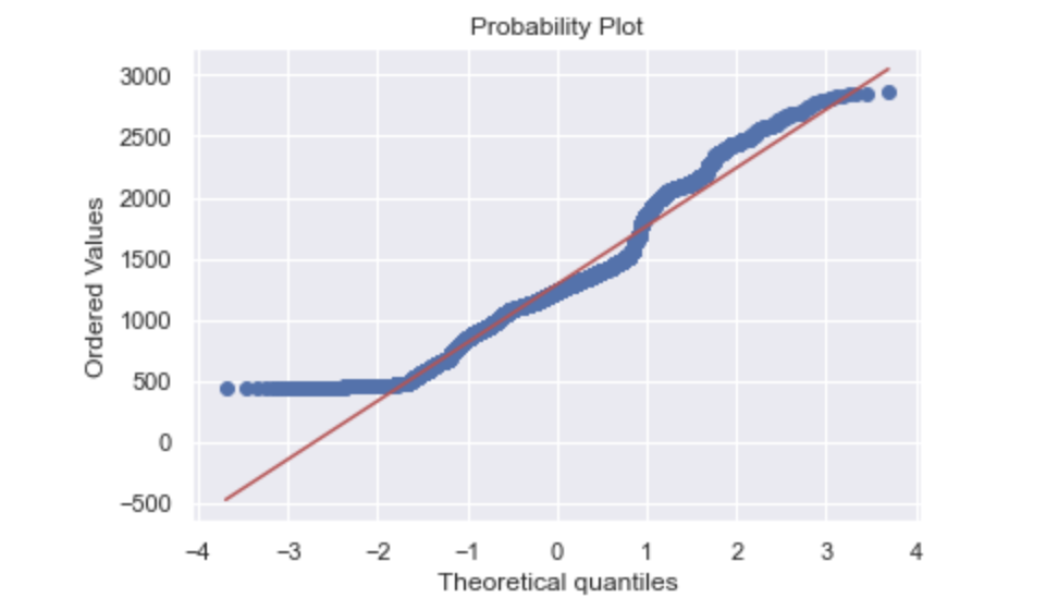
Explanation:

• QQ plot takes all the values and arranges them in accending order.
• y represents how many standard deviations away from the mean
• The red diagonal line represents what the data points should follow if they are Normal Distributed
• In this case, since more values are arond 500, the data is not normally distributed
  • and we cannot use the elegant statistics of Normal Distributions to make successful forecasts

Extra Step: Scrape the real-time data off of Yahoo Finance

 1
 2
 3
 4
 5
 6
 7
 8
 9
10
11
12
13
14
15
16
17
18
19
20
21
22
23
24
25
26

import yfinance
import warnings
warnings.filterwarnings("ignore")

# using the .download() method to scrape our data from the Yahoo Finance webpage
raw_data = yfinance.download(tickers = "^GSPC ^FTSE ^N225 ^GDAXI", start = "1994-01-07", end = "2021-09-20", interval = "1d", group_by = "ticker", auto_adjust = True, treads = True)
# tickers => the time series we are interested in
# interval => the distance in time between two recorded observations. Since we're using daily closing prices, we set it equal to "1d", which indicates 1 day.
# group_by => the way we want to group the scraped data. Usually we want it to be "ticker", so that we have all the information about a time series in 1 variable
# auto_adjuest => Automatically adjust the closing prices for each period
# treads => whether to use threads for mass downloading

df_comp = raw_data.copy()

df_comp['market_value'] = df_comp['^GSPC'].Close

del df_comp['^N225']
del df_comp['^GSPC']
del df_comp['^GDAXI']
del df_comp['^FTSE']
df_comp = df_comp.asfreq('b')
df_comp = df_comp.fillna(method='ffill')

train_size = int(len(df_comp)*0.8)
df_train, df_test  = df_comp.iloc[:train_size], df_comp.iloc[train_size:]

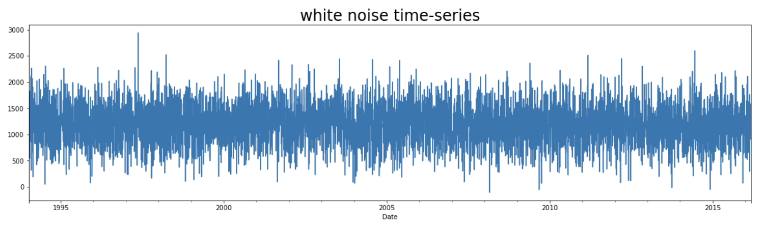
3. White Noise

Definition: A sequence of random data, where every value has a time-period associated with it

• it behaves sporadically, not predictable

Conditions:

• constant mean $\mu$
• constant variance $\sigma^2$
• no autocorrelation in any period: NO clear relationship between past and present values
  • autocorrelation measures how correlated a series is with past versions of itself
  • $\rho = corr(x_t,x_{t-1})$

Generate White Noise data and plot its values

• compare with the graph of the S&P closing prices

1
2
3
4

import matplotlib.pyplot as plt
df_train.wn.plot(figsize = (20,5))
plt.title("white noise time-series", size=24)
plt.show()

Output:

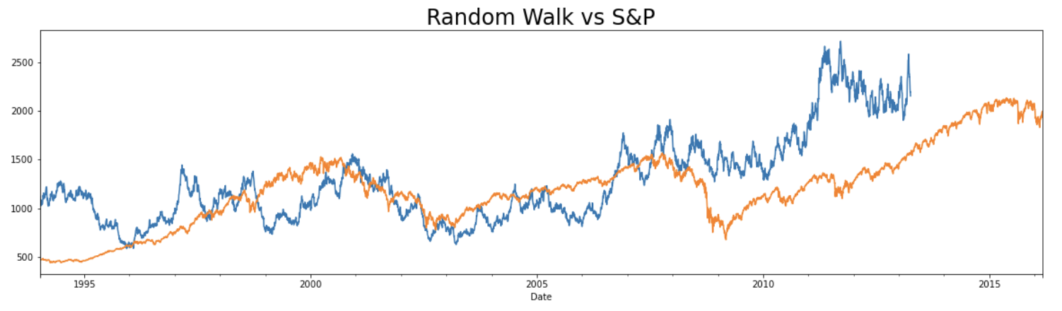
4. Random Walk

Definition: A special type of time-series, where values tend to persist over time and the differences between periods are simply white noise

• $P_t = P_{t-1} + \epsilon_t$, where the residual $\epsilon_t \sim WN(\mu,\sigma^2)$

The random walk data is much more similar to S&P prices than to white noise values

• both have small variations between consecutive time periods
• both have cyclical increases and decreases in short periods of time

 1
 2
 3
 4
 5
 6
 7
 8
 9
10

rw = pd.read_csv("RandWalk.csv")
rw.date = pd.to_datetime(rw.date, dayfirst = True)
rw.set_index("date", inplace = True)
rw = rw.asfreq('b')
df_train['rw'] = rw.price

df_train.rw.plot(figsize = (20,5))
df_train.market_value.plot()
plt.title("Random Walk vs S&P", size = 24)
plt.show()

Output:

Market Efficiency: measures the level of difficulty in forecasting correct future values

• in general, if a time series resembles a random walk, the prices can’t be predicted with great accuracy
• conversely, if future prices can be predicted with great accuracy, then there are arbitrage opportunities
  • we can speak of arbitrage when investors manage to buy and sell commodities and make a safe profit while the price adjusts
  • if such opportunities exist within a market, investors are bound to take advantage, which would eventually lead to a price that matches the expected one, as a result, prices adjust accordingly

5. Stationarity

Strict Stationarity

Rarely observed in nature

• $(x_t,x_{t+k}) \sim Dist(\mu, \sigma^2)$
• $(x_{t+a},x_{t+a+k}) \sim Dist(\mu, \sigma^2)$

Weak-form/Covariance Stationarity

Assumptions:

• Constant $\mu$
• Constant $\sigma^2$
• $Cov(x_n,x_{n+k}) = Cov(x_m, x_{m+k})$
  • consistent covariance between periods at an identical distance

Dickey-Fuller Test: to check whether a data set comes from a stationary process

• Null Hypothesis: assumes non-stationarity
  • autocorrelation coefficient $\varphi < 1$
• Alternative Hypothesis: $\varphi = 1$
• reject the Null if test statistic < critical value in the D-F Table
  • stationarity

 1
 2
 3
 4
 5
 6
 7
 8
 9
10
11
12
13
14
15
16
17
18
19
20
21
22
23
24
25
26
27
28
29
30
31
32
33
34
35
36
37
38
39
40

import statsmodels.graphics.tsaplots as sgt
import statsmodels.tsa.stattools as sts

sts.adfuller(df_train.market_value)

'''
(-0.9614956416665502,        # test statistic is greater than the 1%, 5%, 10% critical values
 0.7670476494835043,         # p-value: there are 76% chance of not rejecting the null (non-stationary process)
 18,                         # there are some autocorrelation going back 18 periods
 5761,                       # number of observations
 {'1%': -3.4314856042568302, # we do not find sufficient evidence of stationary in the data set
  '5%': -2.862041828874895,
  '10%': -2.567037121608915},
 46348.31943803983)          # maximized information criteria provided, lower value => easier to predict the future
'''
# white noise has p-value = 0 => Covariance Stationarity
sts.adfuller(df_train.wn)
'''
(-30.308232415812835,
 0.0,
 6,
 5773,
 {'1%': -3.4314832426913315,
  '5%': -2.8620407854868493,
  '10%': -2.5670365661831696},
 84971.11094405118)
'''

# random walk seems to be a non-stationary process
sts.adfuller(df_train.rw)
'''
(-1.3286073927689719,     # greater than critical values
 0.6159849181617385,
 24,
 4996,
 {'1%': -3.4316595802782865,
  '5%': -2.8621186927706463,
  '10%': -2.567078038881065},
 46299.333497595144)
'''

6. Seasonality

Trends will appear on a cyclical basis.

Ways to test for seasonality:

• Decompose the sequence by splitting the time series into 3 effects:
  • Trend: represents the pattern consistent throughout the data and explains most of the variability of the data
  • Seasonal: expresses all cyclical effects due to seasonality
  • Residual: the difference between true values and predictions for any period

Naive Decomposition： Decomposition function uses the previous period values as a trend-setter.

• Additive: observed = trend + seasonal + residual
• Multiplicative: observed = trend x seasonal x residual

1
2
3
4
5

from statsmodels.tsa.seasonal import seasonal_decompose
import matplotlib.pyplot as plt
season_decomp_additive = seasonal_decompose(df_train.market_value, model = "additive")
season_decomp_additive.plot()
plt.show()

Both Output:

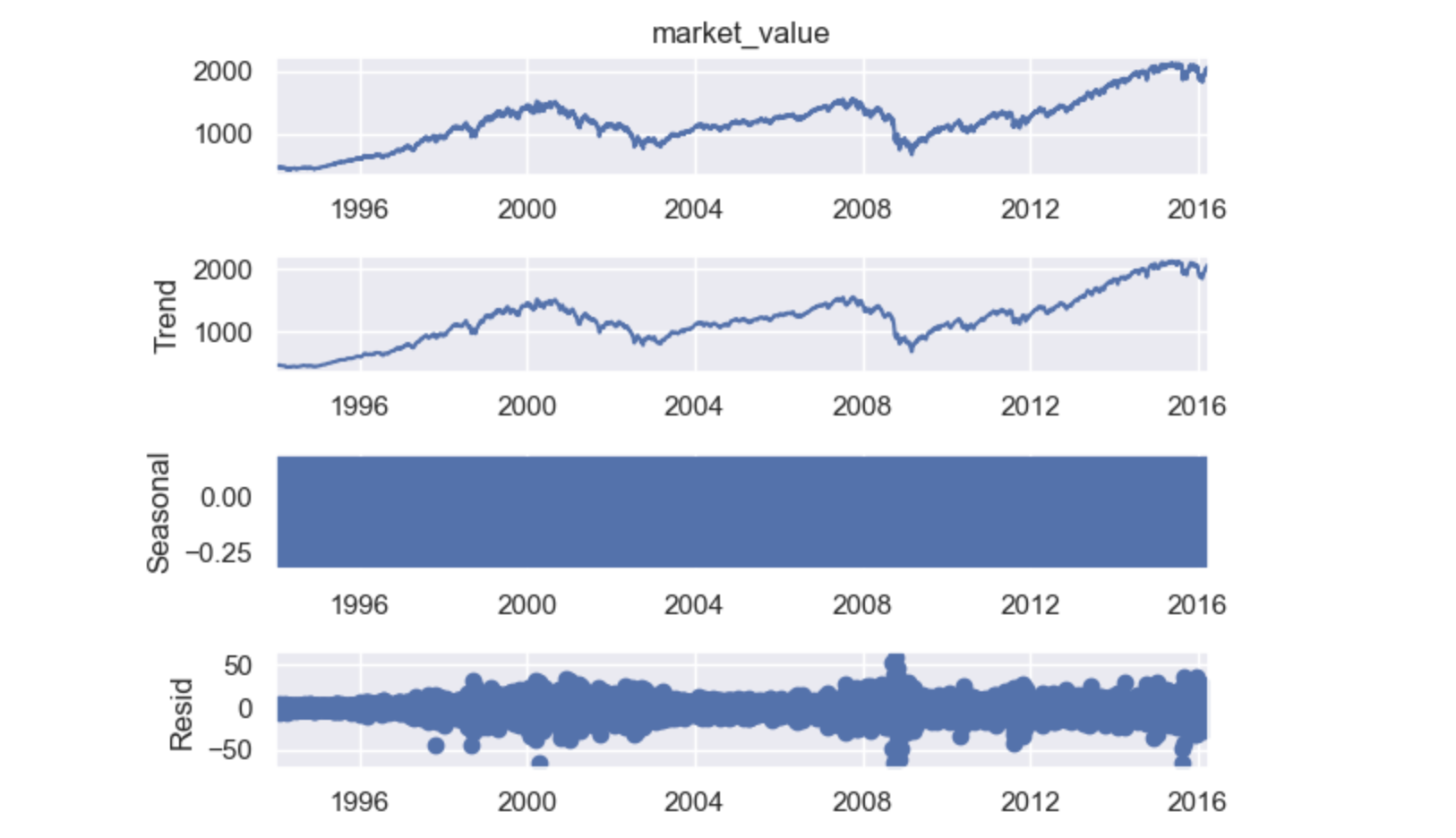
The residuals vary greatly around 2000 and 2008,

• this can be explained by the instability caused by the .com and housing prices bubbles respectively

Seasonal looks like a rectangle:

• values are constantly oscillating back and forth and the figure size is too small
• no concrete cyclical pattern
  • => no seasonality in the S&P data

7. The Autocorrelation Function (ACF)

Correlation measures the similarity in the change of values of two series

• $\rho(x,y)$ only have a single variable

Autocorrelation is the correlation between a sequence and itself

• measures the level of resemblance between a sequence from several periods ago and the actual data
• Lagged is a delayed series of the original one
• how much of yesterday’s values resemble today’s values, or similarities from year to year

ACF for S&P market value

1
2
3
4
5
6
7

import statsmodels.graphics.tsaplots as sgt
sgt.plot_acf(df_train.market_value, zero = False)
# In time series analysis, common practice dictates analyzing the first 40 lags
# zero: Flag indicating whether to include the 0-lag autocorrelation. Default is True.
## indicates whether we include current period values in the graph
plt.title("ACF S&P", size = 24)
plt.show()

Output:

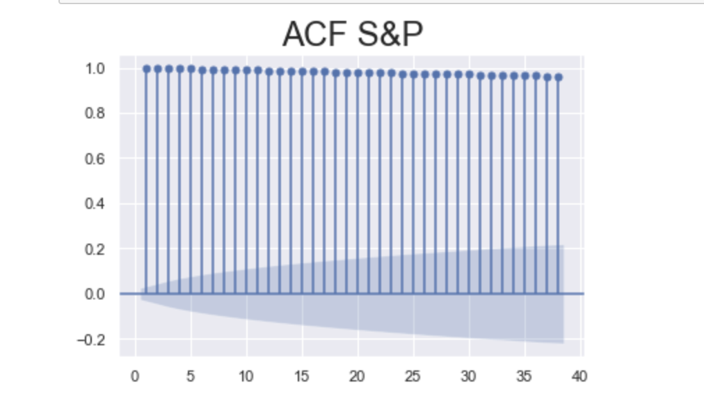
Explanation:

• x-axis: represents lags,
• y-axis: indicates the possible values for the autocorrelation coefficient
• correlation can only take values between -1 and 1,
• lines across the plot represent the autocorrelation between the time series and a lagged copy of itself
• the first line represents the autocorrelation coefficient for one time period ago
• the blue area around the x-axis represents significance, the values situated outside are significantly different from zero which suggests the existence of autocorrelation for that specific lag
• the greater the distance in time, the more UNLIKELY it is that this autocorrelation persists
  • e.g. today’s prices are usually closer to yesterday’s prices than the prices a month ago
• therefore, we need to make sure the autocorrelation coefficient in higher lags is sufficiently greater to be significantly different from zero
• notice how all the lines are positive and higher than the blue region, this suggests the coefficients are significant, which is an indicator of time dependence in the data
  • also, we can see that autocorrelation barely diminishes as the lags increase, this suggests that prices even a month back (40 days ago) can still serve as decent estimators for tomorrow

ACF for White Noise

1
2
3

sgt.plot_acf(df_train.wn, zero = False)
plt.title("ACF WN", size = 24)
plt.show()

Output:

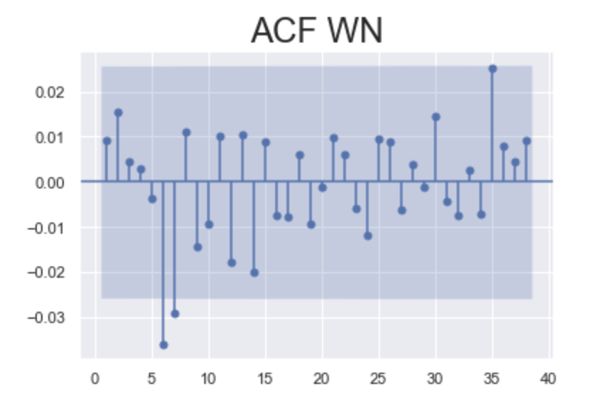
Explanation:

• Since white noise series is generated randomly
  • there are patterns of positive and negative autocorrelation
• All the lines fall within the blue area, thus the coefficients are NOT significant across the entire plot
  • No autocorrelation for any lag

8. The Partial Autocorrelation Function (PACF)

ACF: Prices 3 days ago,

• affecting values of 1 and 2 days ago, which in turn affect present prices indirectly
• affecting present prices directly

PACF cancels out ALL additional channels a previous period value affects the present one

• $X_{t-2}$ => $X_t$
• Cancel Out: $X_{t-2}$ => $X_{t-1}$ => $X_t$

1
2
3

sgt.plot_pacf(df_train.market_value, zero = False, method = ('ols'))
plt.title("PACF S&P", size = 24)
plt.show()

Output:

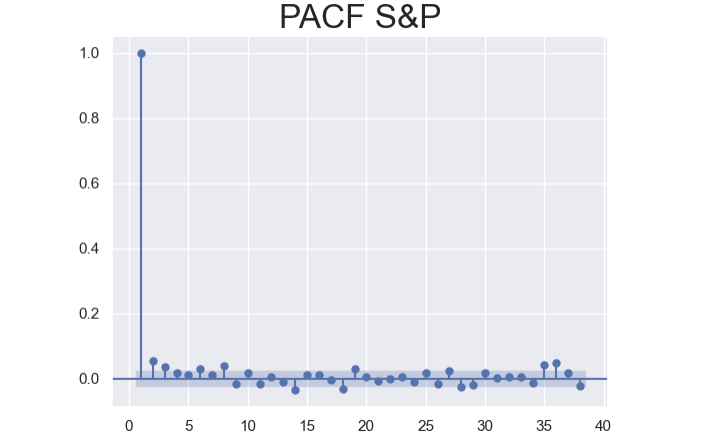
Explanation:

• PACF and ACF values for the first lag should be indentical
• Not significantly different from 0 except the first several lags
  • a tremendous contrast to the ACF plot (all 40 lags are significant)
• Being positive or negative is somewhat random without any lasting effects
  • negative values may be caused from Weekends.

9. The Autoregressive (AR) Model

Autoregressive Model is a linear model, where current period values are a sum of past outcomes multiplied by a numeric factor

• “autoregressive” because the model uses a lagged version of itself (auto) to conduct the regression
• use PACF to select the correct AR model because it shows the individual direct effect each past value has on the current one
• AR(2): $x_{t} = C + \phi_1 x_{t-1} + \phi_2 x_{t-2} + \epsilon_t$
• $ -1 < \phi < 1 $
• $\epsilon_t$: Residuals represent the unpredictable differences between our prediction for period “t” and the correct value
• More lags -> More complicated model -> more coefficients -> some of them are more likely not significant

Fitting an AR(1) Model for Index Prices

Fitting the model: Find the most appropriate coefficients

1
2
3
4
5
6
7
8
9

from statsmodels.tsa.arima_model import ARMA
'''
Parameters:
  order: The (p,d,q) order of the model for the autoregressive, residual values, and moving average components.

'''
model_ar = ARMA(df.market_value, order = (1,0))
results_ar = model_ar.fit()
results_ar.summary()

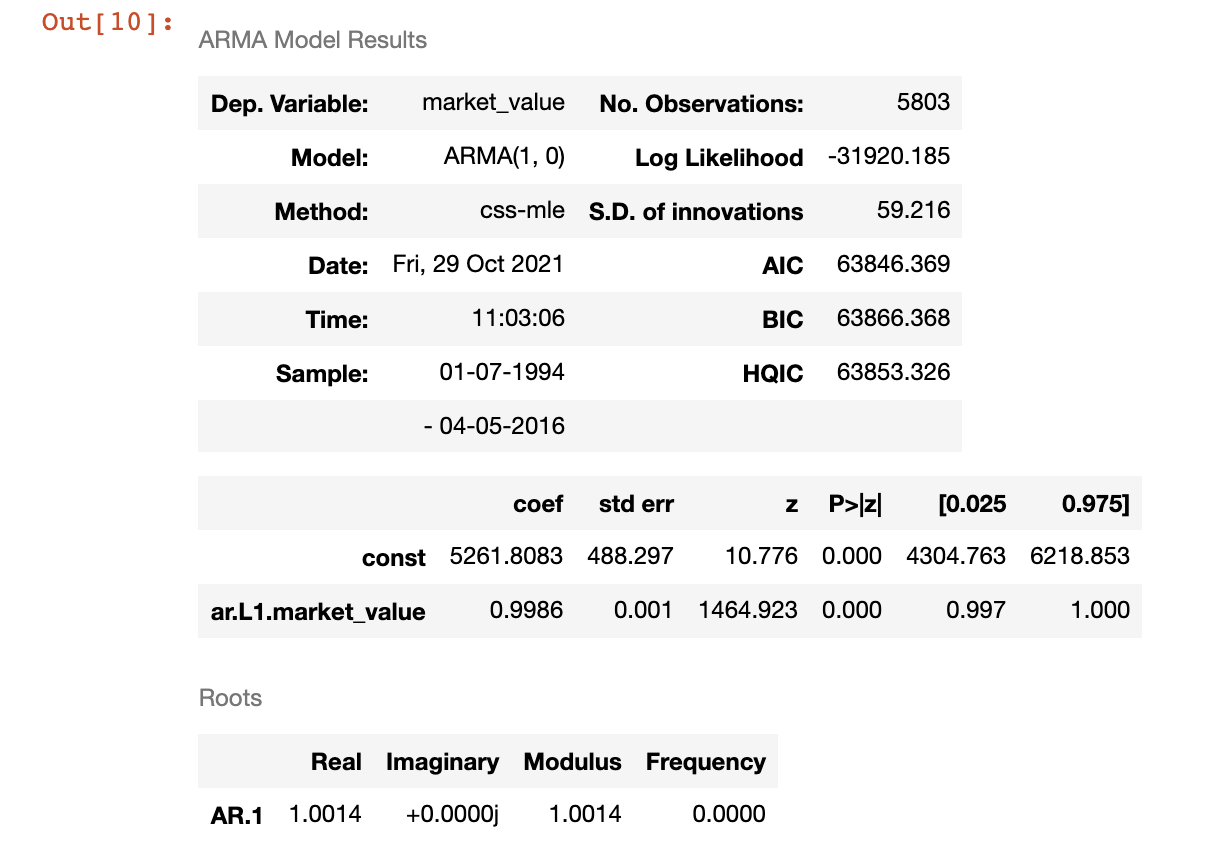
Explanation:
For AR(1) Model: $x_{t} = C + \phi_1 x_{t-1} + \epsilon_t$

• C = 5261.8083
• $\phi_1$ = 0.9986
• std error represents how far away, on average, the model’s predictions are from the true values
• p = 0 means that the coefficients are significantly different from zero

Fitting Higher-Lag AR Models and LLR

Fit AR(2) Model: $x_t = C + \phi_1 x_{t-1} + \phi_2 x_{t-2} + \epsilon_t$

1
2
3

model_ar_2 = ARMA(df.market_value, order = (2,0))
results_ar_2 = model_ar_2.fit()
results_ar_2.summary()

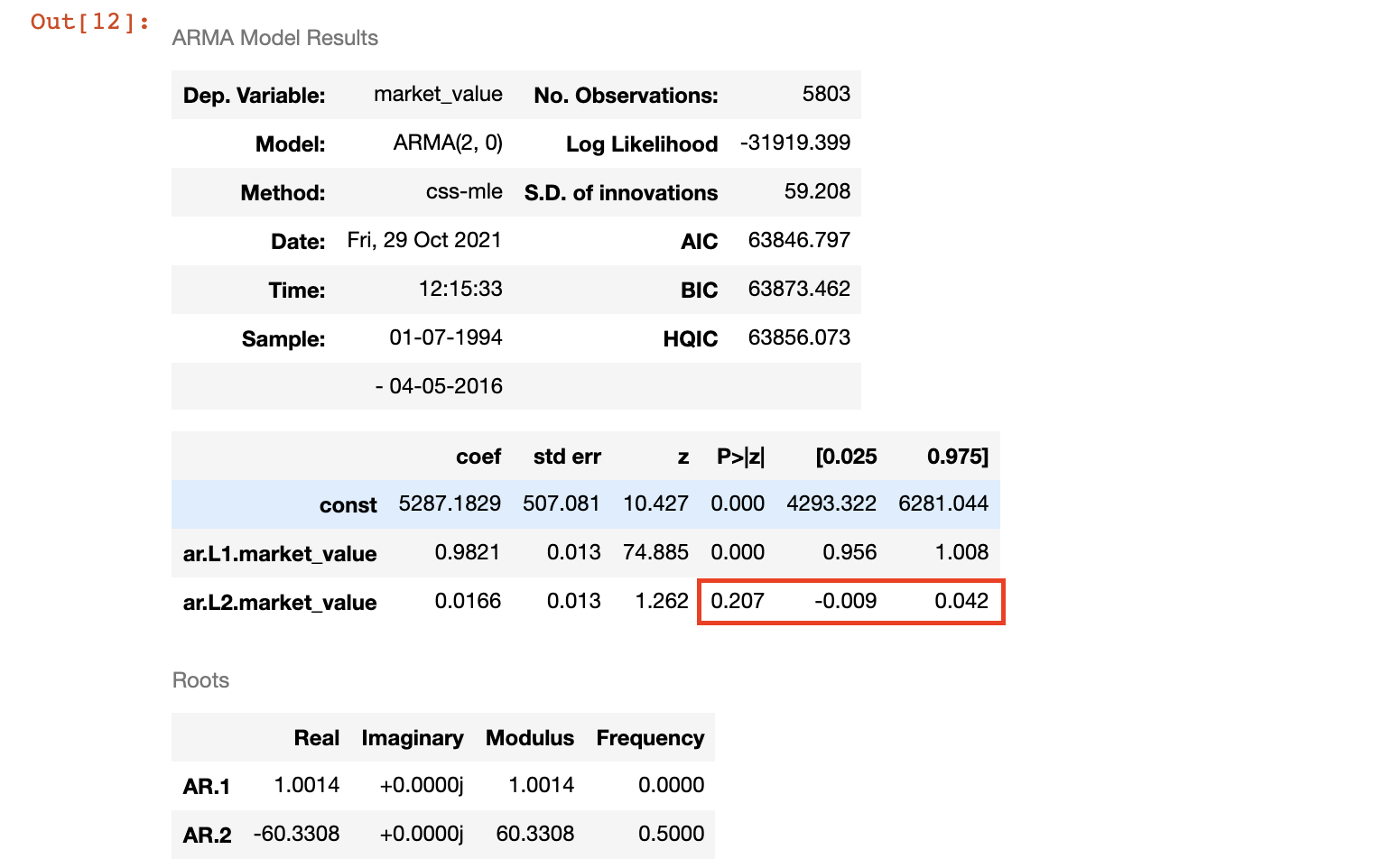
• p = 0.226 > 0.05, reject the H0, $\phi_2$ is NOT significantly different from 0
  • the prices two days ago do not significantly affect today’s prices

Fit AR(3) Model:

• ar.L2.market_value from 0.0166 to -0.0292
  • its p-value 0.112 is still greater than 0.05
• Log Likelihood from -31919.399 to -31913.087
  • higher Log-Likelihood => Lower Information criterion (AIC, BIC, HQIC)

Use Log-Likelihood Ratio (LLR) Test to determine whether a more complex model makes better predictions

 1
 2
 3
 4
 5
 6
 7
 8
 9
10

from scipy.stats import chi2
def LLR_test(mod_1, mod_2, DF=1):
    L1 = mod_1.fit().llf
    L2 = mod_2.fit().llf
    LR = (2*(L2 - L1))
    p = chi2.sf(LR,DF).round(3)
    return p

LLR_test(model_ar_2, model_ar_3) # Return 0.0
LLR_test(model_ar_3, model_ar_4) # Return 0.0

Fitting more complicated models and checking if it gives us Distinguishably Greater Log-Likelihood, then stop before the model that satisfies:

• Non-significant p-value for the LLR Test (> 0.05)
• Non-significant p-value for the highest lag coefficient

1
2
3
4
5

# Fit model_ar_5,6,7 and get significant p-value, higher Log-Likelihhod and lower Information Criteria
model_ar_8 = ARMA(df.market_value, order=(8,0))
results_ar_8 = model_ar_8.fit()
print(results_ar_8.summary())
print("\nLLR Test p-value = " + str(LLR_test(model_ar_7, model_ar_8)))

Output:

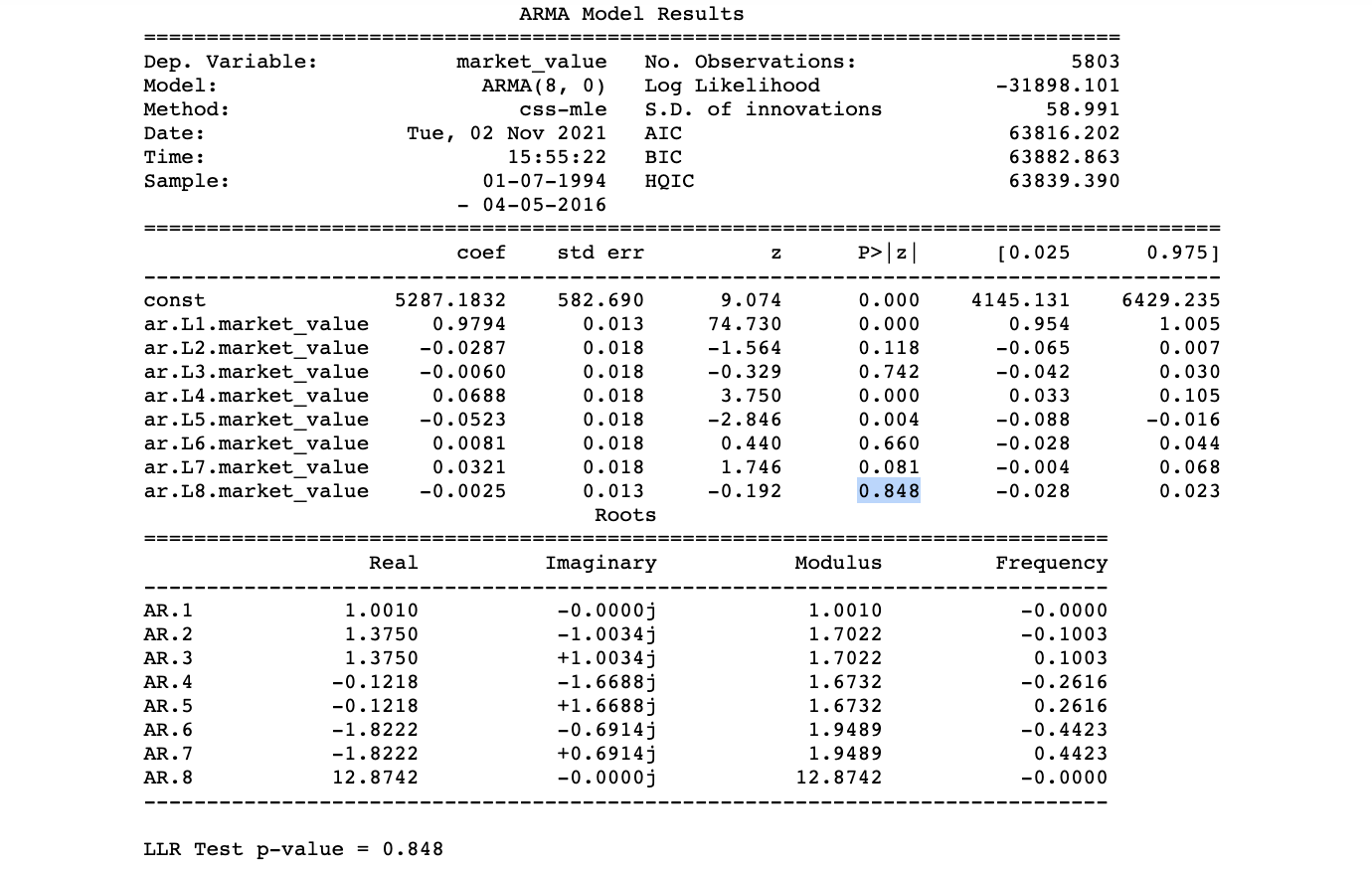
Explanation:

• AR(8) fails the LLR Test => does NOT provide significantly higher Log-Likelihood
• AR(8) has higher Information Criteria
• Including prices from eight periods ago does NOT improve the AR model
• We stop with the AR(7), even though it may contain some non-significant values

Using Returns instead of Prices

Since the market_value extracted from a non-stationary process (by DF-Test)

• we shouldn’t rely on AR Models to make accurate forecasts
• Solution: transform the data set, so that it fits the stationary assumptions
  • the common approach is to use returns instead of prices when measuring financial indices
  • returns: the % change (percentage values) between the values for two consecutive periods

 1
 2
 3
 4
 5
 6
 7
 8
 9
10
11
12
13

df['returns'] = df.market_value.pct_change(1).mul(100)
df = df.iloc[1:] # the first one is Null
sts.adfuller(df.returns)
'''
(-14.549198252857844,    # test statistic is smaller than the 1% critical value
 4.998853863158876e-27,  # p-value <<< 0.05 => stationary
 34,
 5767,
 {'1%': -3.431484422245044,
  '5%': -2.862041306637962,
  '10%': -2.567036843607018},
 17870.834869069306)
'''

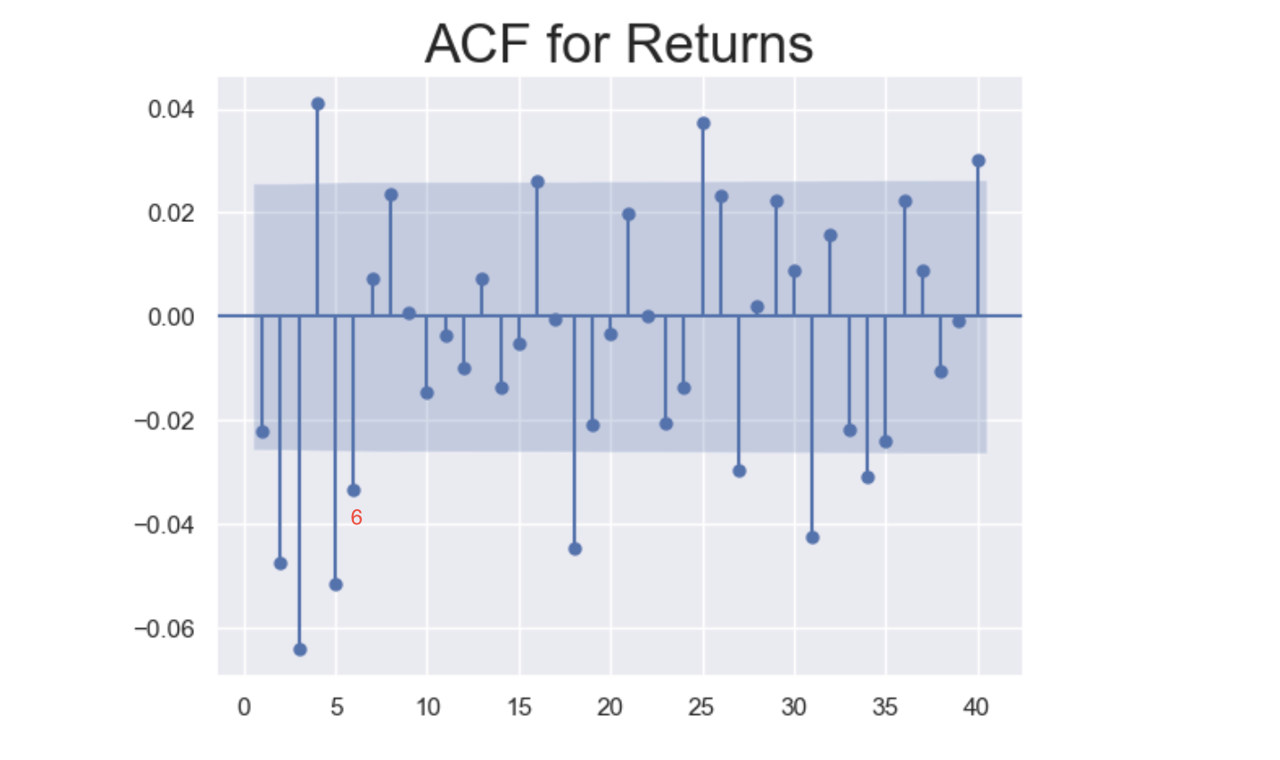
ACF and PACF of Returns

1
2
3
4

fig, (ax1, ax2) = plt.subplots(1, 2, figsize=(9, 4), tight_layout=True)
sgt.plot_acf(df.returns, ax = ax1, lags = 40, title = "ACF of FTSE Returns",zero = False)
sgt.plot_pacf(df.returns, ax = ax2,lags = 40, title = "PACF of FTSE Returns",zero = False, method = ('ols'))
plt.show()

Output:

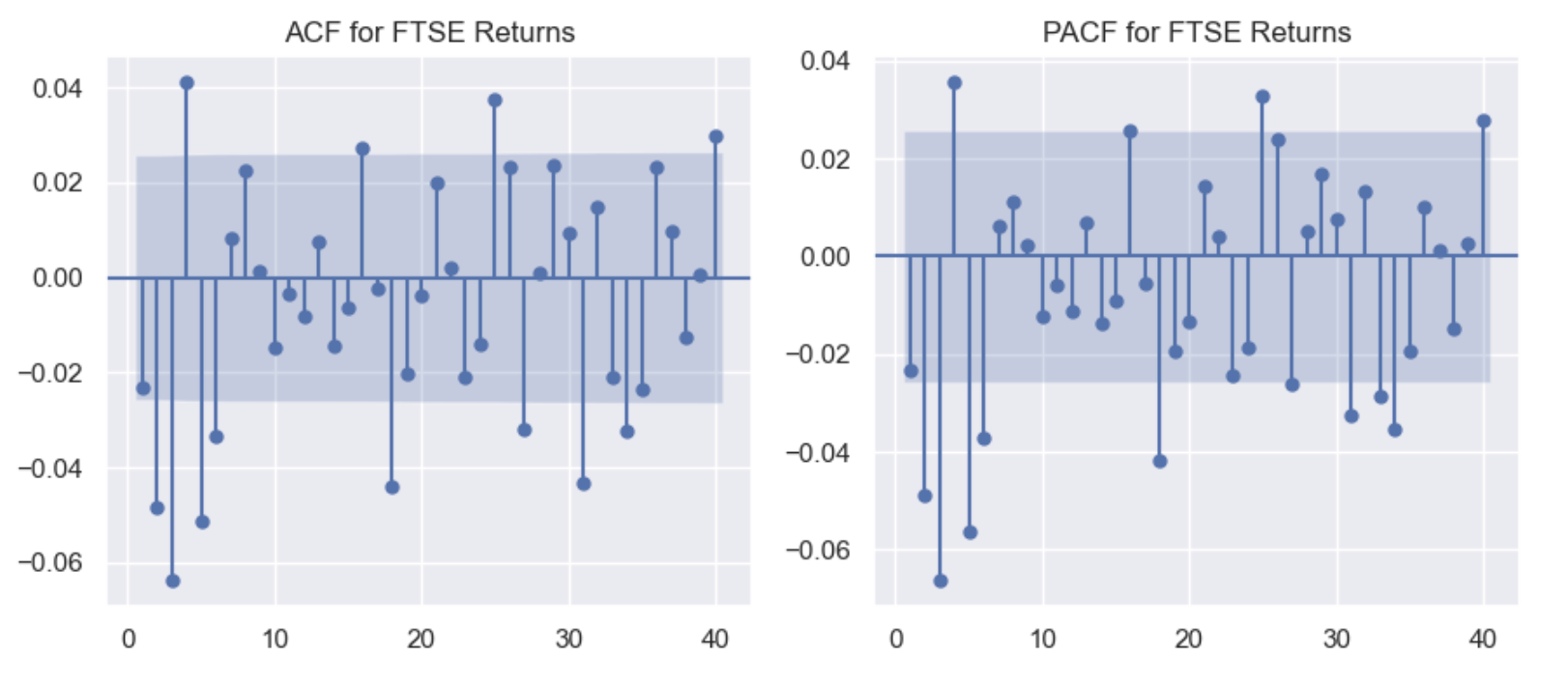
Explanation:

• ACF: Not ALL coefficients are positive or significant (as ACF for Prices)
  • values greatly vary in magnitude instead of being close to 1
• Consecutive values move in different directions
  • this suggests that returns over the entire week are relevant to those of the current one
  • negative relationship may have some form of natural adjustment occuring in the market
    • to avoid falling in a big trend (avoid clustering)
• PACF: Prices today often move in the opposite direction of prices yesterday
  • Price increases following price decreases
• The majority of effects they have on current values should already be accounted for

Fitting an AR(1) Model for Returns

 1
 2
 3
 4
 5
 6
 7
 8
 9
10

model_ret_ar_1 = ARMA(df.returns, order = (1,0))
results_ret_ar_1 = model_ret_ar_1.fit()
results_ret_ar_1.summary()
# p-value for constant: 0.265
# p-value for ar.L1.returns:  0.077 > 0.05

# Neither coefficients is significantly different from 0
# This AR(1) Model holds no real predictive power
# The more easily yesterday's price is affected by higher lags,
# the more inaccurate its coefficient becomes.

Fitting an Higher-Lag AR Model For Returns

1
2
3
4
5
6
7

# Fit model_ret_ar_2,3,4,5,6,
# The more complicated model provides significantly greater Log-Likelihood to justify its greater complexity
model_ret_ar_7 = ARMA(df.returns, order=(7,0))
results_ret_ar_7 = model_ret_ar_7.fit()
print(results_ret_ar_7.summary())
print("\nLLR Test p-value = " + str(LLR_test(model_ret_ar_6, model_ret_ar_7)))
# 0.633, higher information criteria, take model_ret_ar_6

Normalizing Values

Map every value of the sample space to the percentage of the benchmark (first value of the set)

• the resulting series is much easier to compare with other Time Series
• this gives us a better understanding of which ones to invest and which ones to avoid

1
2
3
4

benchmark = df.market_value.iloc[0]
df['norm'] = df.market_value.div(benchmark).mul(100)
sts.adfuller(df.norm)
# p-value = 0.23, smaller than non-normalized prices, but still => non-stationary

Suppose historically, the S&P provides significantly higher returns (3%) than NIKKEI (which yields a steady 2% increase over a given period)

• then if both returns are around 3% for the period we are observing, NIKKEI is significantly outperforming its expectations

To avoid any biased comparision when analyzing the two sets, we often rely on normalized returns

• which account for the absolute profitability of the investment in contrast to prices
• they allows to compare the relative profitability as opposed to non-normalized returns

1
2
3

bench_ret = df.returns.iloc[0]
df['norm_ret'] = df.returns.div(bench_ret).mul(100)
sts.adfuller(df.norm_ret)

• Normalizing does NOT affect stationarity and model selection

Analysing the Residuals

Ideally, the residuals should follow a Random Walk Process, so they should be stationary

Residuals of Prices

1
2
3
4
5
6

df['res_price'] = results_ar_7.resid
df.res_price.mean() # 0.53671587730958 => 0, which suggests that on average, our model performs well
df.res_price.var() # 3479.256211055214 => high variance indicates the Residuals are not concentrated around the mean
# Use DF Test to check stationarity
sts.adfuller(df.res_price) # test statistics = -76.16262235181671 < critical values
# p-value = 0  => stationary

Residuals for Return

1
2
3
4

df['res_ret'] = results_ret_ar_6.resid
print(df.res_ret.mean()) # -4.143527999821654e-05 => 0
print(df.res_ret.var())  # 1.293500958426552 => 1
sts.adfuller(df.res_ret) # p-value = 0, residuals stationary

ACF of Residuals

Recall: the coefficients for the ACF of White Noise should ALL be 0

• Examine the ACF of the Residuals from a fitted model to make sure the errors of predictions are Random
• if the residuals are non-random, then there is a pattern that needs to be accounted for

1
2
3

sgt.plot_acf(df.res_price, zero = False, lags = 40)
plt.title("ACF of Residuals for Prices", size = 24)
plt.show()

Output:

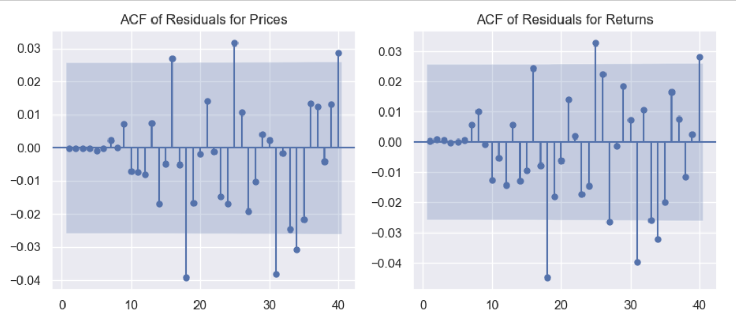
Explanation:

• The majority of coefficients fall within the blue region
  • NOT significantly different from 0, which fits the characteristics of white noise
• The few points outside the blue area lead us to believe there's a better predictor

Unexpected Shocks from Past Periods

AutoRegressive Models need time to adjust from a Big, Unexpected Shock

• because AR models rely on past data, regardless of how close predictions are

There are Self-Correcting Models that take into account past residuals, adjust to unexpected shocks more quickly

• because the predictions are corrected immediately following a big error
• the more errors examined, the more adapted model is to handle unforeseen errors

Moving Average(MA) Models perform well at predicting Random Walk datasets

• because they always adjust from the error of the previous period
• because absorbing shocks allows the mean to move accordingly

This gives the model prediction a much greater chance to move in a similar direction to the values it is trying to predict

• it also stops the model from greatly diverging, which is useful for non-stationary data

10. The Moving Average (MA) Model

$$r_t = c + \theta_1\epsilon_{t-1}+\epsilon_t$$

• $|\theta_n| < 1$ to prevent compounded effects exploding in magnitude
• $\epsilon_t$ and $\epsilon_{t-1}$: Residuals for the current and past period

A Simple MA Model is equivalent to an infinite AR model with certain restrictions

• difference: MA models determine the maximum amount of lags based on ACF (AR models rely on PACF)
  • becaused the MA models aren’t based on past period returns
  • determine which lagged values have a significant direct effect on the present-day ones is NOT relevant

1. Fitting a MA(1) Model for Returns

1
2
3
4

model_ret_ma_1 = ARMA(df.returns[1:], order=(0,1))
# order = (AR components, MA components)
results_ret_ma_1 = model_ret_ma_1.fit()
results_ret_ma_1.summary()

Output:

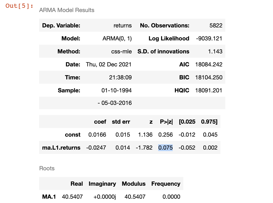
Explanation:

The coefficient for the one-lag-ago residual is significant at 0.10 significant level but not significant 0.05 level

• since the first coefficient of the ACF for Returns is NOT significantly different from 0 (within the blue area)

2. Fitting Higher-Lag MA Models

 1
 2
 3
 4
 5
 6
 7
 8
 9
10
11
12
13
14
15
16
17
18
19
20
21
22
23
24
25
26
27
28
29

# MA(2) Model
model_ret_ma_2 = ARMA(df.returns[1:], order=(0,2))
results_ret_ma_2 = model_ret_ma_2.fit()
print(results_ret_ma_2.summary())
print("\nLLR test p-value = " + str(LLR_test(model_ret_ma_1, model_ret_ma_2)))
# p-values for ma.L2.returns = 0 and ma.L1.returns = 0.023, both significant
# Lower IC
# MA(2) is better than MA(1)

# MA(3)
model_ret_ma_3 = ARMA(df.returns[1:], order=(0,3))
results_ret_ma_3 = model_ret_ma_3.fit()
print(results_ret_ma_3.summary())
print("\nLLR test p-value = " + str(LLR_test(model_ret_ma_2, model_ret_ma_3)))
# p-values for ma.L2.returns = 0 and ma.L3.returns = 0, both significant
# Lower IC
# MA(3) is better than MA(2)

# MA(6) > MA(5) > MA(4) > MA(3)
# because of lower IC and significant LLR test p-value

# MA(7)
model_ret_ma_7 = ARMA(df.returns[1:], order=(0,7))
results_ret_ma_7 = model_ret_ma_7.fit()
print(results_ret_ma_7.summary())
print("\nLLR test p-value = " + str(LLR_test(model_ret_ma_6, model_ret_ma_7)))
# p-value = 0.683
# MA(7) < MA(6)
# Take MA(6) Model

ACF for Returns can give us some hints:

3. Examining the MA Model’s Residuals

We estimate the Standard Deviation of the residual, we can know how far off we can hypothetically be with our predictions

• using the 3 standard deviations rule, we can get a good idea of what interval 99.7% of the data will fall into

1
2
3
4
5
6
7

# Start by extracting the MA(6) Residuals
df['res_ret_ma_6'] = results_ret_ma_6.resid[1:]
print(round(df.res_ret_ma_6.mean(),3)) # Mean = 0
print(round(df.res_ret_ma_6.var(),3))  # Variance = 1.291
df.res_ret_ma_6[1:].plot(figsize = (20,5))
plt.title("MA Model Residuals of Returns", size = 24)
plt.show()

Output:

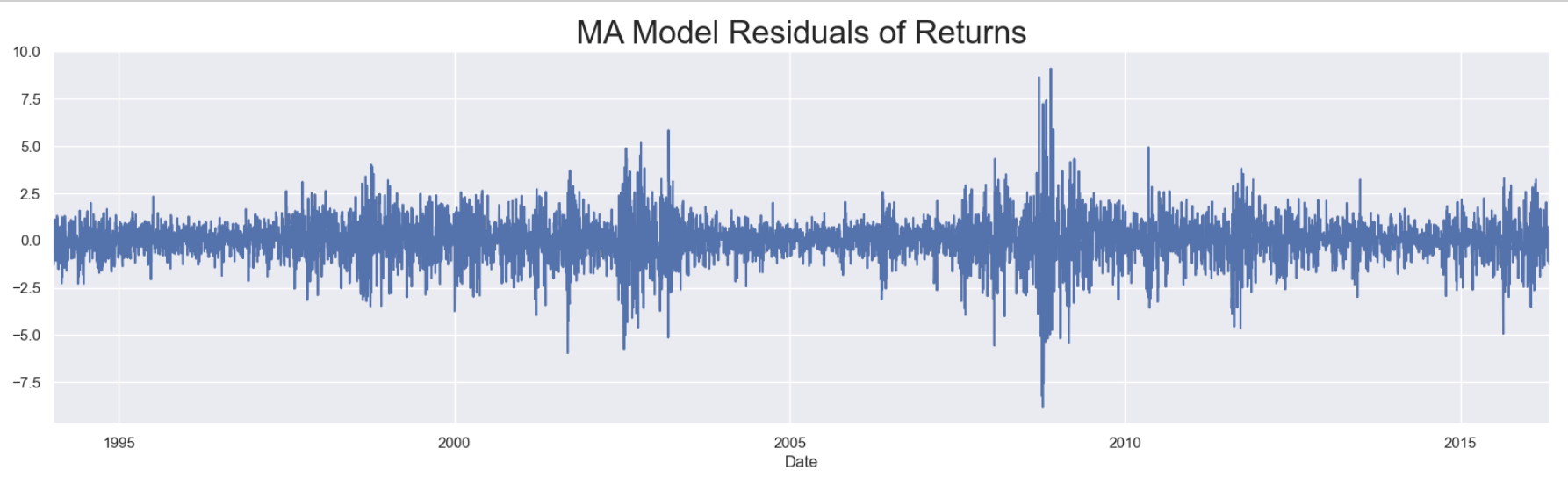
Exclude the .com and house price bubbles, the residuals are random

• to test if the residuals resemble a white noise process, we can check for stationary
• if the data is non-stationary, it can’t be considered white noise

 1
 2
 3
 4
 5
 6
 7
 8
 9
10
11

sts.adfuller(df.res_ret_ma_6[2:])
'''
(-76.28833323226722,
 0.0,   # p-value = 0 => the Residuals are Stationary
 0,
 5820,
 {'1%': -3.4314740870339353,
  '5%': -2.8620367403219062,
  '10%': -2.5670344128257816},
 17915.49917726831)
'''

Check ACF

• since a white noise process produces completely random data
• so that ACF coefficients should NOT be significantly different from zero

1
2
3

sgt.plot_acf(df.res_ret_ma_6[2:], zero = False, lags = 40)
plt.title("ACF of MA Model Residuals for Returns", size = 24)
plt.show()

Output:

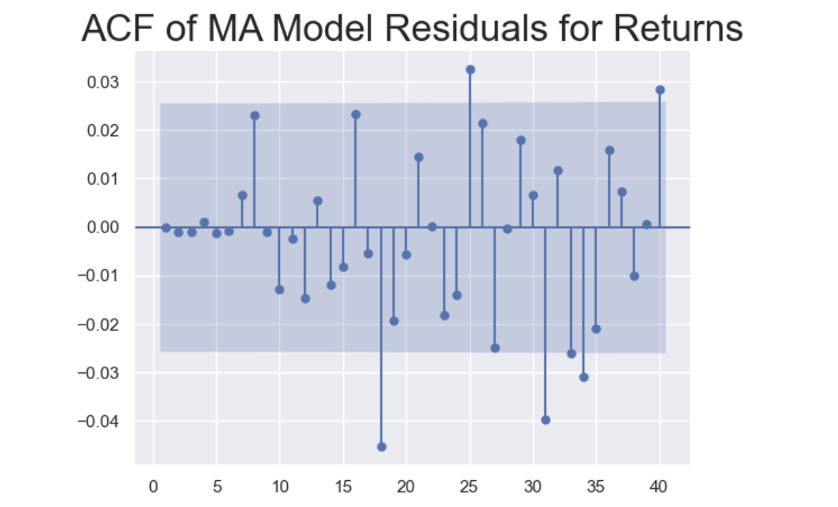
Explanation:
None of the first 17 lags are significant

• the first 6 coefficients are incorporated into the MA Model, so they are close to 0.
• the following 11 insignificant lags show that how well MA(6) model perform

Markets adjust to shocks, so values and errors far in the past lose relevance

• the ACF suggests that the residual data resembles white noise, which means the errors don’t follow a pattern

4. MA Model Selection for Normalized Returns

To compare different market indexes, using the normalized values is important

5. MA Model for Non-Stationary Prices

AR models are less reliable when estimating non-stationary prices