Deep Learning Notes 03 | Regularize Deep Neural Network

2022-01-20 1643 words 8 minutes

Contents

Regularize Deep Neural Networks

这篇笔记记录了深度神经网络的正则化，在【统计学习笔记 03 世上没有解千愁的酒】中，我记录了“没有任何一种模型或算法可以在各种数据集中完胜其它所有的算法，解决所有的问题”，当我们把神经网络的层数加深，神经元节点变多，使其能“深度学习”更多的更复杂的更灵活的非线性函数的同时，也使得模型产生了**过拟合(overfit)**问题 —— 酗酒(overdrink)看似可以完全地麻痹自己让自己完全忘记了所有问题、幻想自己活在了一个完美的温柔乡(low training set error)，但酒醒之后却仍然无力解决任何现实的问题，仍然脆弱至极连站都站不起来更不要说能跑起来(high testing set error)。我们需要自律，深度神经网络亦如是 —— 正则化(Regularization)的加入使得神经网络避免陷入过度拟合的泥沼，在这篇笔记提到的四种正则化的方法(L2, Dropout, Data Augment, Early Stop)可以让其在测试集中表现的仍然良好。

1. Train/Dev/Test Sets

Applying Machine Learning is highly iterative process

Idea ==> Code ==> Experiment
We have to go through the loop many times to figure out your hyperparameters.

We build a model upon training set then optimize hyperparameters on dev set as much as possible.

finally evaluate the model on testing set.

Traditional Split:

60/20/20 for Train/Dev/Test Sets

For big data (> 1,000,000):

99/1/1 because 1% x 1000000 = 10000 is enough for dev and test
The trend now gives the training data the biggest sets.

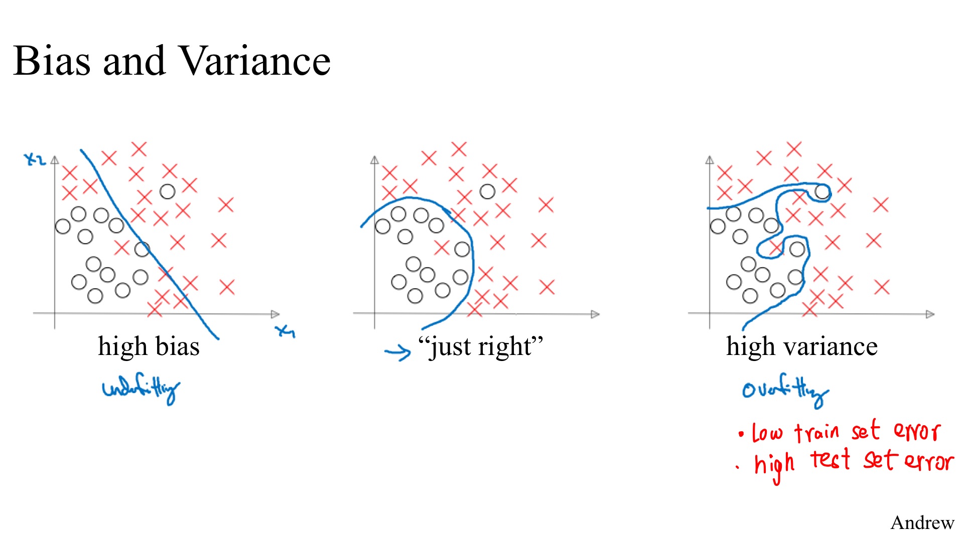
2. Bias/Variance Tradeoff

Basic Recipe for Machine Learning:

Check whether there is High Bias first (training data performance), if so:

Bigger Network with more layers or more hidden units
Train longer
Try different optimization algorithm
Try different Neural Network Architecture that is more suitable for the data or the problem

Check whether there is High Variance (test set performance), if so:

give more data (expensive sometimes)
NN architecture search
Regularization

3. Regularization

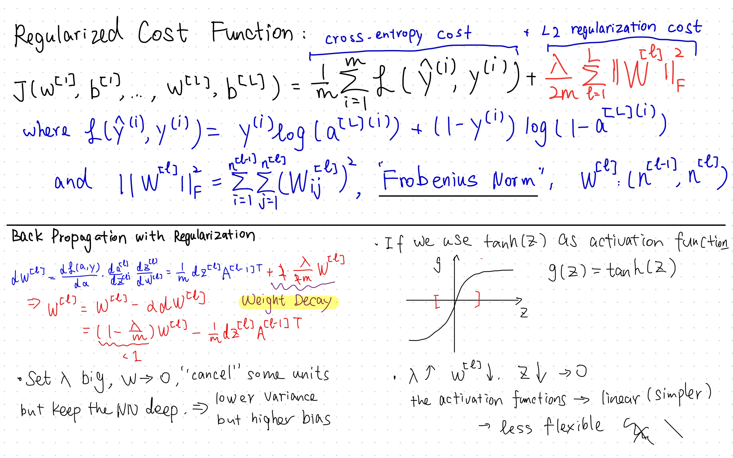
3.1. L2 Regularization

L2-regularization relies on the assumption that a model with small weights is simpler than a model with large weights.

Thus, by penalizing the square values of the weights in the cost function you drive all the weights to smaller values.
It becomes too costly for the cost to have large weights! This leads to a smoother model in which the output changes more slowly as the input changes.
L2 regularization makes your decision boundary smoother. If λ is too large, it is also possible to “oversmooth”, resulting in a model with high bias.
The value of λ is a hyperparameter that you can tune using a dev set.

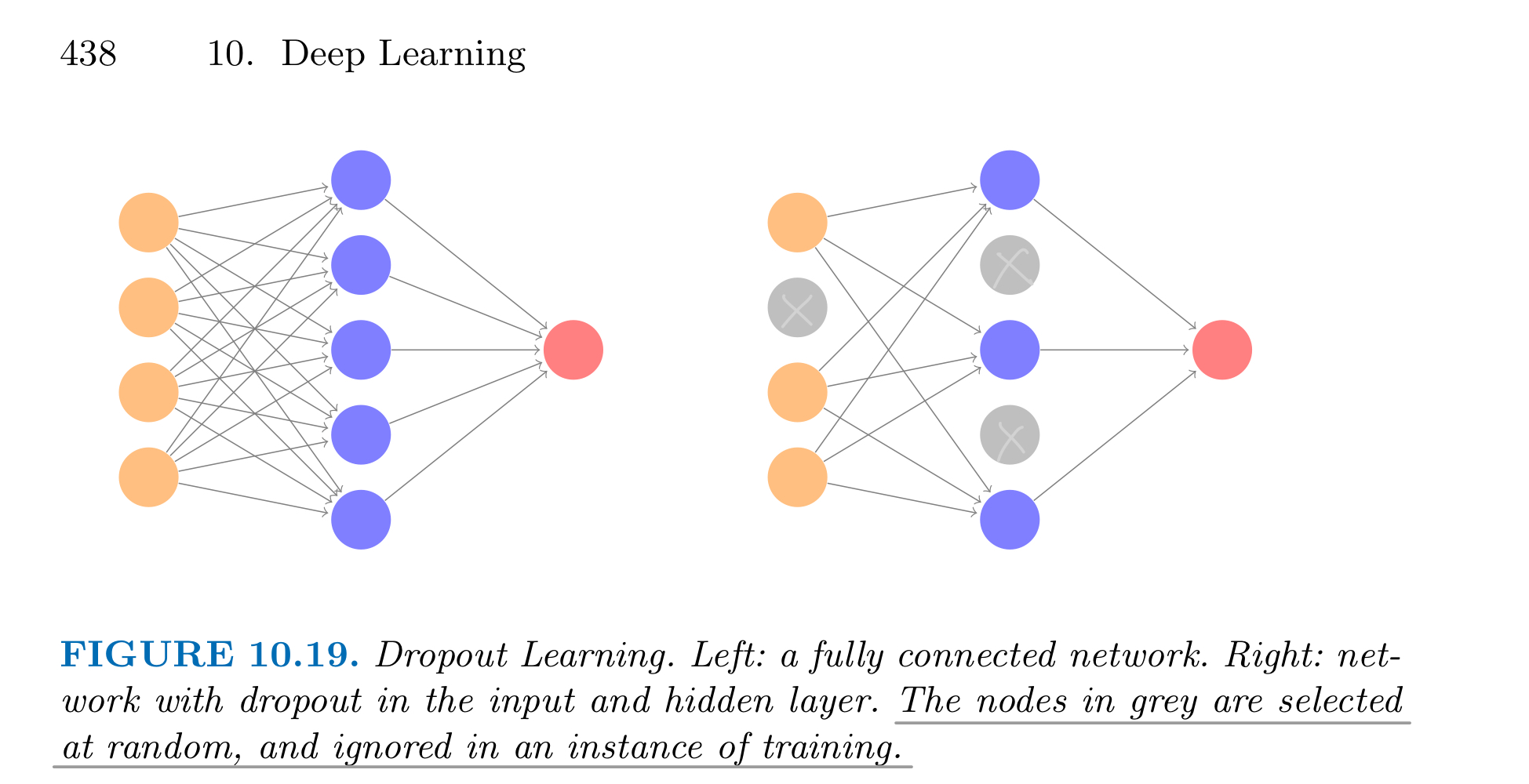
3.2. Dropout (10.7.3)

Inspired by Random Forest (Section 8.2), the idea is to randomly remove a fraction of the units in a layer when fitting the model.

this prevents nodes from becoming over-specialized, similiar in some respects to ridge regularization (Section 6.2.1.)

A lot of researchers are using dropout with Computer Vision (CV) because they have a very big input size and almost never have enough data, so overfitting is the usual problem. And dropout is a regularization technique to prevent overfitting.

A downside of dropout is that the cost function J is not well defined and it will be hard to debug (plot J by iteration).

The “inverted-dropout” method:

 1
 2
 3
 4
 5
 6
 7
 8
 9
10


keep_prob = 0.8   # 0 <= keep_prob <= 1
l = 3  # this code is only for layer 3
# the generated number that are less than 0.8 will be dropped. 80% stay, 20% dropped
d3 = np.random.rand(a[l].shape[0], a[l].shape[1]) < keep_prob

a3 = np.multiply(a3,d3)   # keep only the values in d3

# increase a3 to not reduce the expected value of output
# (ensures that the expected value of a3 remains the same) - to solve the scaling problem
a3 = a3 / keep_prob

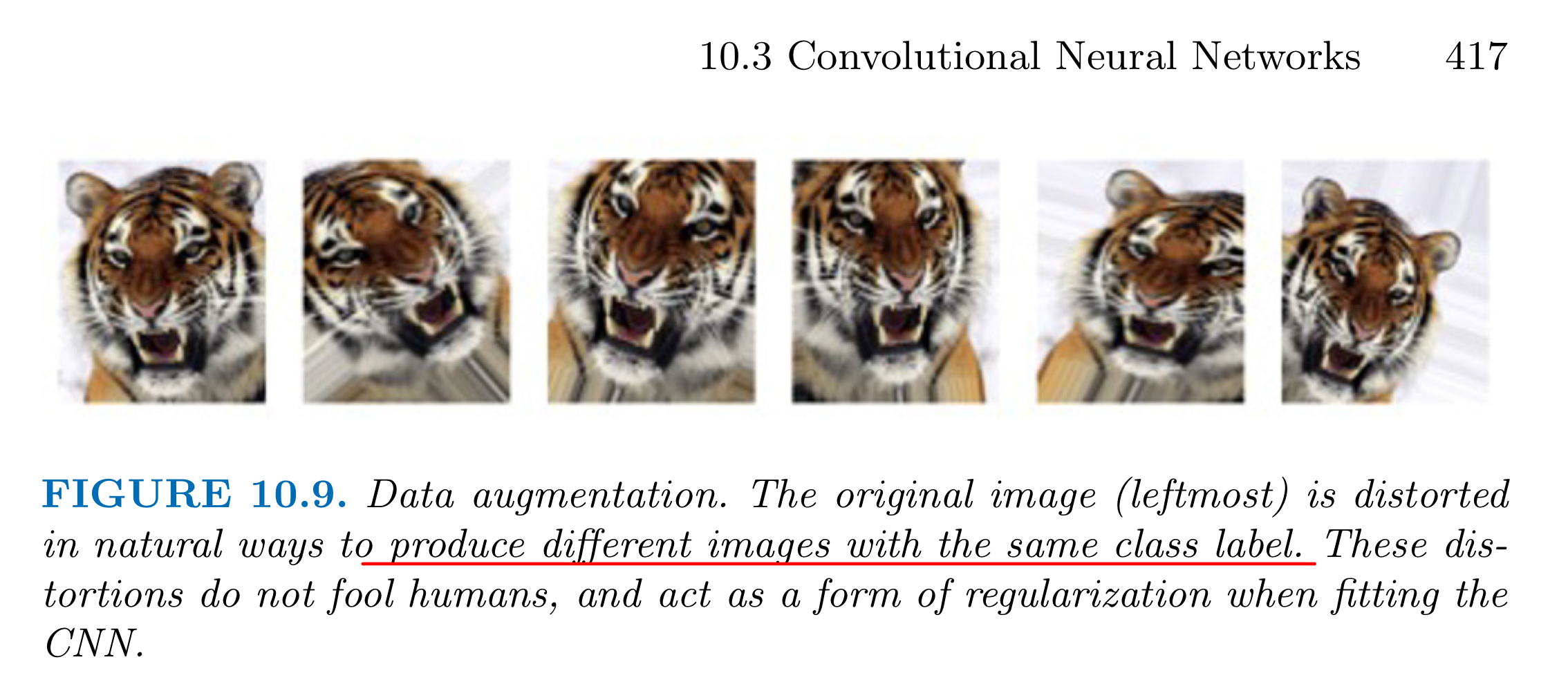
3.3. Data Augmentation (10.3.4)

Getting more new training data might be expensive, however, each old training image could be replicated many times, with each replicate randomly distorted in a natural way,

such as zoom, horizontal and vertical shift, shear, small rotations and flip.
Data Augmentation protects against overfitting, this kind of fattening of the data is similiar in spirit to ridge regularization.

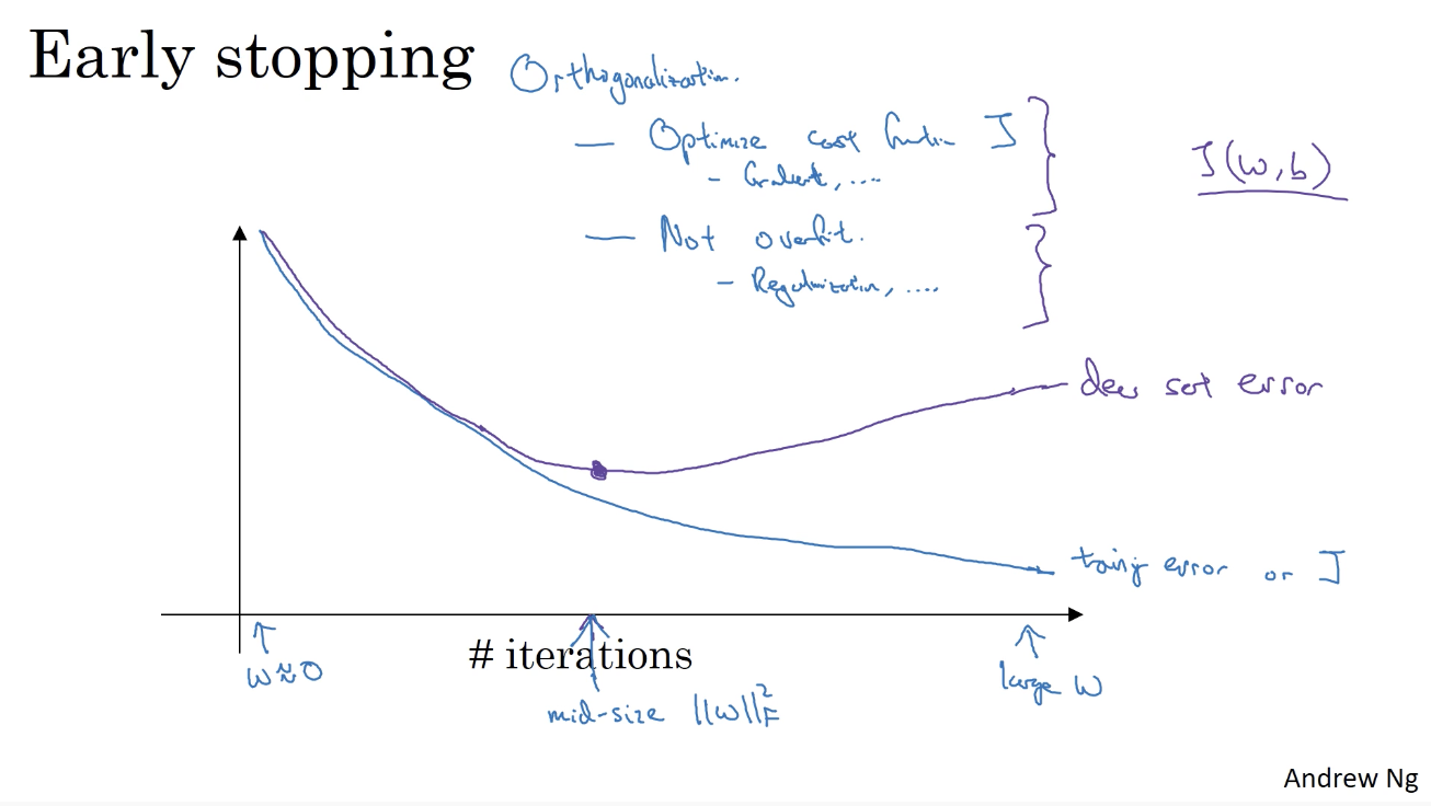
3.4. Early Stop and Normalize the Input

Early Stopping during Stochastic Gradient Descent (SGD) can serve as a form of regularization that prevents us from interpolating the training data, while still getting very good results on test data.

plot the training set and the dev set cost together for each iteration.
- At some iteration the dev set cost will stop decreasing and will start increasing.
stop and pick the point at which the training set error and dev set error are best (lowest training cost with lowest dev cost), to avoid overfitting.

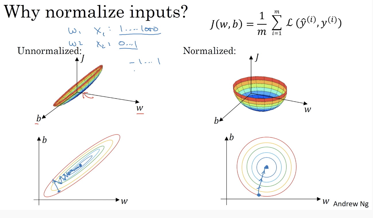
Normalizing the input is a way to keep input X (and its weight W) consistent and speed up the gradient descent

If we don’t normalize the inputs, the cost function J will be deep and its shape will be inconsistent (elongated) then optimizing it will take a long time.

4. Code Implementation

4.1. L2 Regularization

 1
 2
 3
 4
 5
 6
 7
 8
 9
10
11
12
13
14
15
16
17
18
19
20
21
22
23
24
25
26
27
28
29
30
31
32
33
34
35
36
37
38
39


def backward_propagation_with_regularization(X, Y, cache, lambd):
    """
    Implements the backward propagation of our baseline model to which we added an L2 regularization.

    Arguments:
    X -- input dataset, of shape (input size, number of examples)
    Y -- "true" labels vector, of shape (output size, number of examples)
    cache -- cache output from forward_propagation()
    lambd -- regularization hyperparameter, scalar

    Returns:
    gradients -- A dictionary with the gradients with respect to each parameter, activation and pre-activation variables
    """

    m = X.shape[1]
    (Z1, A1, W1, b1, Z2, A2, W2, b2, Z3, A3, W3, b3) = cache

    dZ3 = A3 - Y

    dW3 = 1./m * np.dot(dZ3, A2.T) + (lambd/m)*W3
    db3 = 1./m * np.sum(dZ3, axis=1, keepdims = True)

    dA2 = np.dot(W3.T, dZ3)
    dZ2 = np.multiply(dA2, np.int64(A2 > 0))

    dW2 = 1./m * np.dot(dZ2, A1.T) + (lambd/m)*W2
    db2 = 1./m * np.sum(dZ2, axis=1, keepdims = True)

    dA1 = np.dot(W2.T, dZ2)
    dZ1 = np.multiply(dA1, np.int64(A1 > 0))

    dW1 = 1./m * np.dot(dZ1, X.T) + (lambd/m)*W1
    db1 = 1./m * np.sum(dZ1, axis=1, keepdims = True)

    gradients = {"dZ3": dZ3, "dW3": dW3, "db3": db3,"dA2": dA2,
                 "dZ2": dZ2, "dW2": dW2, "db2": db2, "dA1": dA1,
                 "dZ1": dZ1, "dW1": dW1, "db1": db1}

    return gradients

4.2. Dropout Regularization

Forward Propagation with Dropout

 1
 2
 3
 4
 5
 6
 7
 8
 9
10
11
12
13
14
15
16
17
18
19
20
21
22
23
24
25
26
27
28
29
30
31
32
33
34
35
36
37
38
39
40
41
42
43
44
45
46
47
48
49
50
51


def forward_propagation_with_dropout(X, parameters, keep_prob = 0.5):
    """
    Implements the forward propagation: LINEAR -> RELU + DROPOUT -> LINEAR -> RELU + DROPOUT -> LINEAR -> SIGMOID.

    Arguments:
    X -- input dataset, of shape (2, number of examples)
    parameters -- python dictionary containing your parameters "W1", "b1", "W2", "b2", "W3", "b3":
                    W1 -- weight matrix of shape (20, 2)
                    b1 -- bias vector of shape (20, 1)
                    W2 -- weight matrix of shape (3, 20)
                    b2 -- bias vector of shape (3, 1)
                    W3 -- weight matrix of shape (1, 3)
                    b3 -- bias vector of shape (1, 1)
    keep_prob - probability of keeping a neuron active during drop-out, scalar

    Returns:
    A3 -- last activation value, output of the forward propagation, of shape (1,1)
    cache -- tuple, information stored for computing the backward propagation
    """

    np.random.seed(1)

    # retrieve parameters
    W1 = parameters["W1"]
    b1 = parameters["b1"]
    W2 = parameters["W2"]
    b2 = parameters["b2"]
    W3 = parameters["W3"]
    b3 = parameters["b3"]

    # LINEAR -> RELU -> LINEAR -> RELU -> LINEAR -> SIGMOID
    Z1 = np.dot(W1, X) + b1
    A1 = relu(Z1)
    D1 = np.random.rand(A1.shape[0], A1.shape[1])     # Step 1: initialize matrix D1 = np.random.rand(..., ...)
    D1 = (D1 < keep_prob).astype(int)                 # Step 2: convert entries of D1 to 0 or 1 (using keep_prob as the threshold)
    A1 = A1*D1                                        # Step 3: shut down some neurons of A1
    A1 = A1/keep_prob                                 # Step 4: scale the value of neurons that haven't been shut down

    Z2 = np.dot(W2, A1) + b2
    A2 = relu(Z2)
    D2 = np.random.rand(A2.shape[0], A2.shape[1])     # Step 1: initialize matrix D2 = np.random.rand(..., ...)
    D2 = (D2 < keep_prob)                             # Step 2: convert entries of D2 to 0 or 1 (using keep_prob as the threshold)
    A2 = A2*D2                                        # Step 3: shut down some neurons of A2
    A2 = A2/keep_prob                                 # Step 4: scale the value of neurons that haven't been shut down

    Z3 = np.dot(W3, A2) + b3
    A3 = sigmoid(Z3)

    cache = (Z1, D1, A1, W1, b1, Z2, D2, A2, W2, b2, Z3, A3, W3, b3)

    return A3, cache

Backward Propagation with Dropout

 1
 2
 3
 4
 5
 6
 7
 8
 9
10
11
12
13
14
15
16
17
18
19
20
21
22
23
24
25
26
27
28
29
30
31
32
33
34
35
36
37
38
39
40
41
42
43


def backward_propagation_with_dropout(X, Y, cache, keep_prob):
    """
    Implements the backward propagation of our baseline model to which we added dropout.

    Arguments:
    X -- input dataset, of shape (2, number of examples)
    Y -- "true" labels vector, of shape (output size, number of examples)
    cache -- cache output from forward_propagation_with_dropout()
    keep_prob - probability of keeping a neuron active during drop-out, scalar

    Returns:
    gradients -- A dictionary with the gradients with respect to each parameter, activation and pre-activation variables
    """

    m = X.shape[1]
    (Z1, D1, A1, W1, b1, Z2, D2, A2, W2, b2, Z3, A3, W3, b3) = cache

    dZ3 = A3 - Y
    dW3 = 1./m * np.dot(dZ3, A2.T)
    db3 = 1./m * np.sum(dZ3, axis=1, keepdims = True)
    dA2 = np.dot(W3.T, dZ3)
    # Step 1: Apply mask D2 to shut down the same neurons as during the forward propagation
    dA2 = dA2*D2
    # Step 2: Scale the value of neurons that haven't been shut down
    dA2 = dA2/keep_prob
    dZ2 = np.multiply(dA2, np.int64(A2 > 0))
    dW2 = 1./m * np.dot(dZ2, A1.T)
    db2 = 1./m * np.sum(dZ2, axis=1, keepdims = True)

    dA1 = np.dot(W2.T, dZ2)
    # Step 1: Apply mask D1 to shut down the same neurons as during the forward propagation
    dA1 = dA1*D1
    # Step 2: Scale the value of neurons that haven't been shut down
    dA1 = dA1/keep_prob
    dZ1 = np.multiply(dA1, np.int64(A1 > 0))
    dW1 = 1./m * np.dot(dZ1, X.T)
    db1 = 1./m * np.sum(dZ1, axis=1, keepdims = True)

    gradients = {"dZ3": dZ3, "dW3": dW3, "db3": db3,"dA2": dA2,
                 "dZ2": dZ2, "dW2": dW2, "db2": db2, "dA1": dA1,
                 "dZ1": dZ1, "dW1": dW1, "db1": db1}

    return gradients