Deep Learning Notes 02 | Deep Neural Network

Yiyang Dong

2022-01-06 1997 words 10 minutes

Contents

4. Deep Neural Networks

Why Deep ?

Logistic Regression and Single Layer Neural Networks perform well on some Simple Binary Classification Problems

Deep Neural Networks (or Deep Learning) can solve more complex problems
Neuroscientists believe that the human brain also starts off detecting simple things like edges to complex things like faces
Layers “learn” simpler functions to more complex functions

Face Detection:

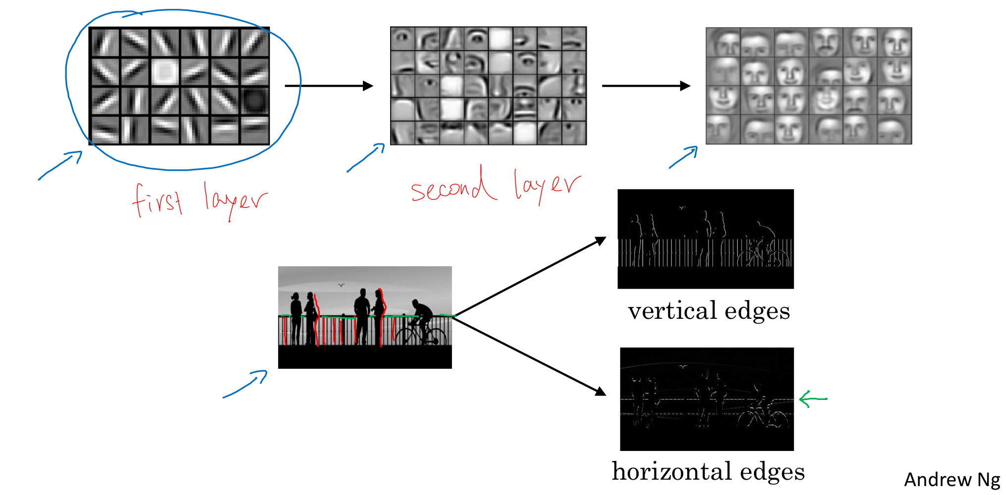
The first layer of the neural network could be considered as Edge Detector
- each hidden unit may figure out different edge orintation (horizontal or vertical edges)
The second layer could group the edges detected in first layer together
- different units may detect different parts of faces (eyes, noses,..)
The third layer could recognize or detect different types of faces

Speech Recognition:

The first layer of the neural network might learn to detect low-level audio waveform features
- up/down tone, white noise,
The second layer learns to detect different basic units of sound (or phoneme)
The third layer may learn to detect words and then sentences…

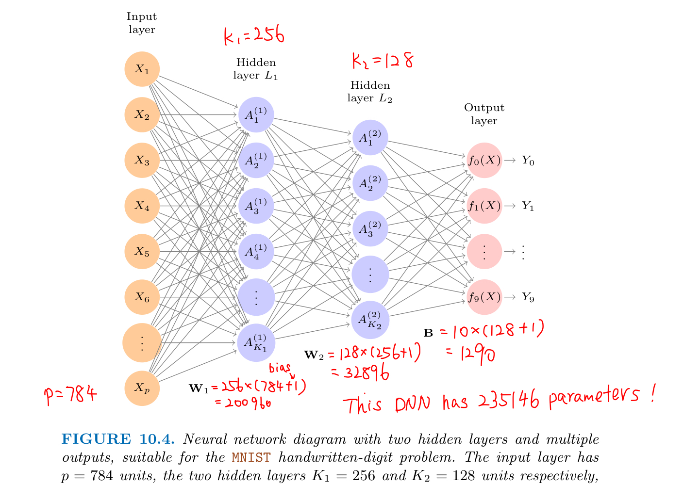
Hand-Written Digit Recognition

The idea is to build a Deep Neural Network to classify the images into their correct digit class 0-9:

each imput vector $X$ stores one image that has p = 28 x 28 = 784 pixels, each of which is an eight-bit grayscale value between 0 and 255
the output is the class label, represented by a vector $Y = (Y_0, Y_1, …, Y_9)$ of 10 dummy variables
- e.g. Y = (0,0,0,0,0,1,0,0,0,0) represents 5
- this is called one-hot encoding in Machine Learning community
it has two hidden layers $L_1$ (256 units) and $L_2$ (128 units)

Build L-Layer DNN

Step 1: Random Initialization

use np.random.randn(layer_dims[l], layer_dims[l-1]) * 0.01

 1
 2
 3
 4
 5
 6
 7
 8
 9
10
11
12
13
14
15
16
17
18
19
20
21
22
23


def initialize_parameters_deep(layer_dims):
    """
    Arguments:
    layer_dims -- python array (list) containing the dimensions of each layer in our network

    Returns:
    parameters -- python dictionary containing your parameters "W1", "b1", ..., "WL", "bL":
                    Wl -- weight matrix of shape (layer_dims[l], layer_dims[l-1])
                    bl -- bias vector of shape (layer_dims[l], 1)
    """

    np.random.seed(3)
    parameters = {}
    L = len(layer_dims)            # number of layers in the network

    for l in range(1, L):
        parameters['W' + str(l)] = np.random.randn(layer_dims[l],layer_dims[l-1]) * 0.01
        parameters['b' + str(l)] = np.zeros((layer_dims[l],1))

        assert(parameters['W' + str(l)].shape == (layer_dims[l], layer_dims[l-1]))
        assert(parameters['b' + str(l)].shape == (layer_dims[l], 1))

    return parameters

Step 2: Forward Propagation

records all intermediate values in “caches”

 1
 2
 3
 4
 5
 6
 7
 8
 9
10
11
12
13
14
15
16
17
18
19
20
21
22
23
24
25
26
27
28
29
30
31
32
33
34
35
36
37
38
39
40
41
42
43
44
45
46
47
48
49
50
51
52
53
54
55
56
57
58
59
60
61
62


def linear_activation_forward(A_prev, W, b, activation):
    """
    Implement the forward propagation for the LINEAR->ACTIVATION layer

    Arguments:
    A_prev -- activations from previous layer (or input data): (size of previous layer, number of examples)
    W -- weights matrix: numpy array of shape (size of current layer, size of previous layer)
    b -- bias vector, numpy array of shape (size of the current layer, 1)
    activation -- the activation to be used in this layer, stored as a text string: "sigmoid" or "relu"

    Returns:
    A -- the output of the activation function, also called the post-activation value
    cache -- a python tuple containing "linear_cache" and "activation_cache";
             stored for computing the backward pass efficiently
    """

    if activation == "sigmoid":
        # Inputs: "A_prev, W, b". Outputs: "A, activation_cache".
        Z, linear_cache = linear_forward(A_prev, W, b) # This "linear_cache" contains (A_prev, W, b)
        A, activation_cache = sigmoid(Z) # This "activation_cache" contains "Z"

    elif activation == "relu":
        # Inputs: "A_prev, W, b". Outputs: "A, activation_cache".
        Z, linear_cache = linear_forward(A_prev, W, b) # This "linear_cache" contains (A_prev, W, b)
        A, activation_cache = relu(Z) # This "activation_cache" contains "Z"

    assert (A.shape == (W.shape[0], A_prev.shape[1]))
    cache = (linear_cache, activation_cache)

    return A, cache

def L_model_forward(X, parameters):
    """
    Implement forward propagation for the [LINEAR->RELU]*(L-1)->LINEAR->SIGMOID computation

    Arguments:
    X -- data, numpy array of shape (input size, number of examples)
    parameters -- output of initialize_parameters_deep()

    Returns:
    AL -- last post-activation value
    caches -- list of caches containing:
                every cache of linear_activation_forward() (there are L-1 of them, indexed from 0 to L-1)
    """

    caches = []
    A = X
    L = len(parameters) // 2                  # number of layers in the neural network

    # Implement [LINEAR -> RELU]*(L-1). Add "cache" to the "caches" list.
    for l in range(1, L):
        A_prev = A
        A, cache = linear_activation_forward(A_prev, parameters['W' + str(l)], parameters['b' + str(l)], "relu")
        caches.append(cache)

    # Implement LINEAR -> SIGMOID. Add "cache" to the "caches" list.
    AL, cache = linear_activation_forward(A, parameters['W' + str(L)], parameters['b' + str(L)], "sigmoid")
    caches.append(cache)

    assert(AL.shape == (1,X.shape[1]))

    return AL, caches

Step 3: Compute the cross-entropy Cost

 1
 2
 3
 4
 5
 6
 7
 8
 9
10
11
12
13
14
15
16
17
18
19
20
21
22
23


def compute_cost(AL, Y):
    """
    Implement the cost function defined by equation (7).

    Arguments:
    AL -- probability vector corresponding to your label predictions, shape (1, number of examples)
    Y -- true "label" vector (for example: containing 0 if non-cat, 1 if cat), shape (1, number of examples)

    Returns:
    cost -- cross-entropy cost
    """

    m = Y.shape[1]

    # Compute loss from aL and y.
    ### START CODE HERE ### (≈ 1 lines of code)
    cost = (-1/m) * (np.dot(Y, np.log(AL).T) + np.dot((1-Y), np.log(1-AL).T))
    ### END CODE HERE ###

    cost = np.squeeze(cost)      # To make sure your cost's shape is what we expect (e.g. this turns [[17]] into 17).
    assert(cost.shape == ())

    return cost

Step 5: Backward Propagation

 1
 2
 3
 4
 5
 6
 7
 8
 9
10
11
12
13
14
15
16
17
18
19
20
21
22
23
24
25
26
27
28
29
30
31
32
33
34
35
36
37
38
39
40
41
42
43
44
45
46
47
48
49
50
51
52
53
54
55
56
57
58
59
60
61
62
63
64
65
66
67
68
69
70
71
72
73
74
75
76
77
78
79
80
81
82
83
84
85
86
87
88
89
90
91
92
93
94


def linear_backward(dZ, cache):
    # Here cache is "linear_cache" containing (A_prev, W, b) coming from the forward propagation in the current layer
    """
    Implement the linear portion of backward propagation for a single layer (layer l)

    Arguments:
    dZ -- Gradient of the cost with respect to the linear output (of current layer l)
    cache -- tuple of values (A_prev, W, b) coming from the forward propagation in the current layer

    Returns:
    dA_prev -- Gradient of the cost with respect to the activation (of the previous layer l-1), same shape as A_prev
    dW -- Gradient of the cost with respect to W (current layer l), same shape as W
    db -- Gradient of the cost with respect to b (current layer l), same shape as b
    """
    A_prev, W, b = cache
    m = A_prev.shape[1]

    dW = (1/m) * np.dot(dZ, A_prev.T)
    db = (1/m) * np.sum(dZ, axis=1, keepdims=True)
    dA_prev = np.dot(W.T,dZ)

    assert (dA_prev.shape == A_prev.shape)
    assert (dW.shape == W.shape)
    assert (db.shape == b.shape)

    return dA_prev, dW, db

def linear_activation_backward(dA, cache, activation):
    """
    Implement the backward propagation for the LINEAR->ACTIVATION layer.

    Arguments:
    dA -- post-activation gradient for current layer l
    cache -- tuple of values (linear_cache, activation_cache) we store for computing backward propagation efficiently
    activation -- the activation to be used in this layer, stored as a text string: "sigmoid" or "relu"

    Returns:
    dA_prev -- Gradient of the cost with respect to the activation (of the previous layer l-1), same shape as A_prev
    dW -- Gradient of the cost with respect to W (current layer l), same shape as W
    db -- Gradient of the cost with respect to b (current layer l), same shape as b
    """
    linear_cache, activation_cache = cache

    if activation == "relu":
        dZ = relu_backward(dA, activation_cache)

    elif activation == "sigmoid":
        dZ = sigmoid_backward(dA, activation_cache)

    dA_prev, dW, db = linear_backward(dZ, linear_cache)


    return dA_prev, dW, db

def L_model_backward(AL, Y, caches):
    """
    Implement the backward propagation for the [LINEAR->RELU] * (L-1) -> LINEAR -> SIGMOID group

    Arguments:
    AL -- probability vector, output of the forward propagation (L_model_forward())
    Y -- true "label" vector (containing 0 if non-cat, 1 if cat)
    caches -- list of caches containing:
                every cache of linear_activation_forward() with "relu" (it's caches[l], for l in range(L-1) i.e l = 0...L-2)
                the cache of linear_activation_forward() with "sigmoid" (it's caches[L-1])

    Returns:
    grads -- A dictionary with the gradients
             grads["dA" + str(l)] = ...
             grads["dW" + str(l)] = ...
             grads["db" + str(l)] = ...
    """
    grads = {}
    L = len(caches) # the number of layers
    m = AL.shape[1]
    Y = Y.reshape(AL.shape) # after this line, Y is the same shape as AL

    # Initializing the backpropagation
    dAL = - (np.divide(Y, AL) - np.divide(1 - Y, 1 - AL))

    # Lth layer (SIGMOID -> LINEAR) gradients. Inputs: "dAL, current_cache". Outputs: "grads["dAL-1"], grads["dWL"], grads["dbL"]
    current_cache = caches[L-1] # Last Layer
    grads["dA" + str(L-1)], grads["dW" + str(L)], grads["db" + str(L)] = linear_activation_backward(dAL, current_cache, "sigmoid")

    # Loop from l=L-2 to l=0
    for l in reversed(range(L-1)):
        # lth layer: (RELU -> LINEAR) gradients.
        # Inputs: "grads["dA" + str(l + 1)], current_cache". Outputs: "grads["dA" + str(l)] , grads["dW" + str(l + 1)] , grads["db" + str(l + 1)]
        current_cache = caches[l]
        dA_prev_temp, dW_temp, db_temp = linear_activation_backward(grads["dA" + str(l + 1)], current_cache, activation = "relu")
        grads["dA" + str(l)] = dA_prev_temp
        grads["dW" + str(l + 1)] = dW_temp
        grads["db" + str(l + 1)] = db_temp

    return grads

Step 6: Update Parameters

 1
 2
 3
 4
 5
 6
 7
 8
 9
10
11
12
13
14
15
16
17
18
19
20
21


def update_parameters(parameters, grads, learning_rate):
    """
    Update parameters using gradient descent

    Arguments:
    parameters -- python dictionary containing your parameters
    grads -- python dictionary containing your gradients, output of L_model_backward

    Returns:
    parameters -- python dictionary containing your updated parameters
                  parameters["W" + str(l)] = ...
                  parameters["b" + str(l)] = ...
    """

    L = len(parameters) // 2 # number of layers in the neural network

    # Update rule for each parameter. Use a for loop.
    for l in range(L):
        parameters["W" + str(l+1)] = parameters["W" + str(l+1)] - learning_rate * grads["dW" + str(l+1)]
        parameters["b" + str(l+1)] = parameters["b" + str(l+1)] - learning_rate * grads["db" + str(l+1)]
    return parameters

Step 7: Integrate DNN Model

 1
 2
 3
 4
 5
 6
 7
 8
 9
10
11
12
13
14
15
16
17
18
19
20
21
22
23
24
25
26
27
28
29
30
31
32
33
34
35
36
37
38
39
40
41
42
43
44
45
46
47
48
49
50
51


def L_layer_model(X, Y, layers_dims, learning_rate = 0.0075, num_iterations = 3000, print_cost=False):#lr was 0.009
    """
    Implements a L-layer neural network: [LINEAR->RELU]*(L-1)->LINEAR->SIGMOID.

    Arguments:
    X -- data, numpy array of shape (num_px * num_px * 3, number of examples)
    Y -- true "label" vector (containing 0 if cat, 1 if non-cat), of shape (1, number of examples)
    layers_dims -- list containing the input size and each layer size, of length (number of layers + 1).
    learning_rate -- learning rate of the gradient descent update rule
    num_iterations -- number of iterations of the optimization loop
    print_cost -- if True, it prints the cost every 100 steps

    Returns:
    parameters -- parameters learnt by the model. They can then be used to predict.
    """

    np.random.seed(1)
    costs = []                         # keep track of cost

    # Parameters initialization
    parameters = initialize_parameters_deep(layers_dims)

    # Loop (gradient descent)
    for i in range(0, num_iterations):

        # Forward propagation: [LINEAR -> RELU]*(L-1) -> LINEAR -> SIGMOID.
        AL, caches = L_model_forward(X, parameters)

        # Compute cost.
        cost = compute_cost(AL, Y)

        # Backward propagation.
        grads = L_model_backward(AL, Y, caches)

        # Update parameters.
        parameters = update_parameters(parameters, grads, learning_rate)

        # Print the cost every 100 training example
        if print_cost and i % 100 == 0:
            print ("Cost after iteration %i: %f" %(i, cost))
        if print_cost and i % 100 == 0:
            costs.append(cost)

    # plot the cost
    plt.plot(np.squeeze(costs))
    plt.ylabel('cost')
    plt.xlabel('iterations (per hundreds)')
    plt.title("Learning rate =" + str(learning_rate))
    plt.show()

    return parameters