Deep Learning Notes 01 | Simple Neural Network

2022-01-05 2036 words 10 minutes

Contents

Index

– Simple NN
– Deep NN
– CNN, U-Net, YOLO
– PointNets ==> 3D object dection
– Pose Estimation

1. Neural Network History

Neural networks rose to fame (成名) in the late 1980s, fall from favor (失宠) because some “new methods” such as SVMs, Boosting, and Random Forests were more automatic and outperformed poorly-trained neural networks on many problems for the first decade in the new millennium (2000 - 2010)

however, neural networks resurfaced after 2010 with the new name deep learning, with new architectures, the availability of ever-larger training datasets,
and a string of success stories on some niche problems such as
- image and video classification (by Convolutional Neural Networks)
- speech and text modeling (by Recurrent Neural Networks)

2. Single Layer Neural Networks (Sec 10.1)

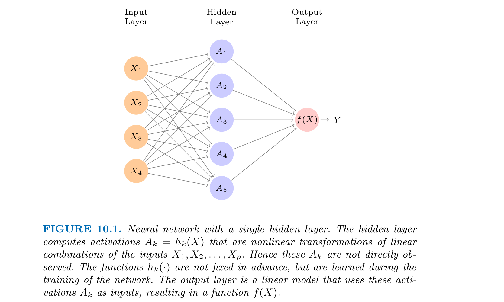
A neural network takes an input vector of p variables, $X = (X_1, X_2, X_3, \cdots, X_p)$, and builds a complex nonlinear function $f(X)$ to predict the response Y.

The name Neural Networks originally derived from thinking of these hidden units as analogous to neurons in the brain:

nodes represent inputs, activations or outputs
edges represent weights or biases
values of the activations $A_k$ close to one are firing, while those close to zero are silent

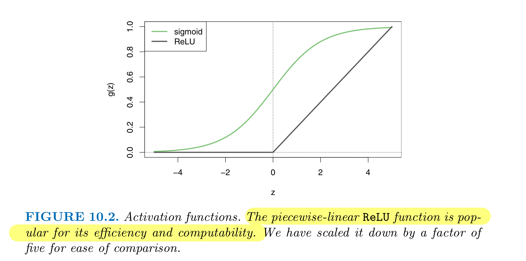
Activation Functions

We can think of each $A_k$ as a different nonlinear transformation of linear combinations of the input features

much like the basis functions (in Sec 7.3) that can be applied to X to fit a non-linear model.
not fixed in advance, but will be learned during the training (computing) of the network.

Why Nonlinear?

otherwise, the neural network is just computing and outputting a linear activation function of the input X
then, the hidden layers are useless.

Rules of Thumb:

Sigmoid activation function can convert a linear function into probabilities between 0 and 1
- only works well in the output layer for Binary Classification (0/1) Problem
tanh activation function works better than the sigmoid function because the mean is close to 0 rather than 0.5
- Centering the Data so that makes the learning for the next layer a litter bit easier
- Disadvantage: if Z is either very large or very small, then the derivative (slope of function) becomes very small
  - this can slow down Gradient Descent
Relu(Rectified Linear Unit) activation function can be computed and stored more efficiently in modern neural networks
- default choice of activation function for hidden layers

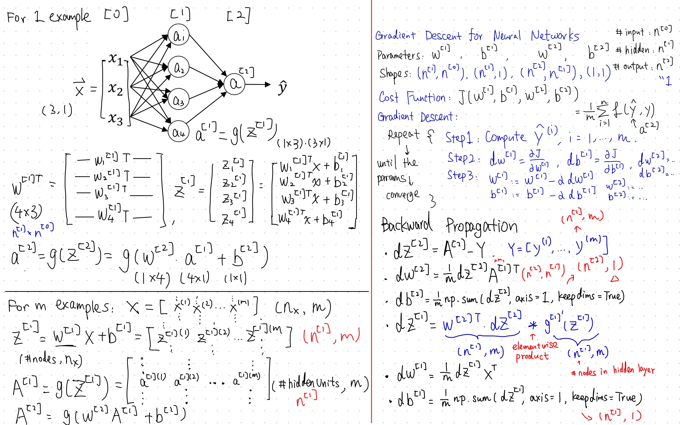
Forward and Backward Propagation

Gradient Descent and Learning Rate

Smaller Learning Rate may make the Gradient Descent Algorithm converge to the minimum:

While a bad Learning Rate causes diverging:

3. Build a Single Layer Neural Network Step by Step

Step 1. Define the Neural Network Structure

Define three variables:

n_x: the size of the input layer (shapes of X)
n_h: the size of the hidden layer (set this to 4)
n_y: the size of the output layer (shapes of Y)

 1
 2
 3
 4
 5
 6
 7
 8
 9
10
11
12
13
14
15
16


def layer_sizes(X, Y):
    """
    Arguments:
    X -- input dataset of shape (input size, number of examples)
    Y -- labels of shape (output size, number of examples)

    Returns:
    n_x -- the size of the input layer
    n_h -- the size of the hidden layer
    n_y -- the size of the output layer
    """
    n_x = X.shape[0] # size of input layer
    n_h = 4
    n_y = Y.shape[0] # size of output layer

    return (n_x, n_h, n_y)

Step 2. Initialize the Parameters

If we initialize weights to 0, all hidden units are completely identical (symmetric)

they compute exact same function
we need to initialize the random and small parameters
- if the weights are too large, then the slope of the gradient will be very small (flat parts of activation functions)

Make sure the parameters' sizes are right

Use np.random.randn(a,b)*0.01 to randomly initialize a matrix of shape (a,b)
Use np.zeros((a,b)) to initialize a matrix of shape (a,b) with zeros.

 1
 2
 3
 4
 5
 6
 7
 8
 9
10
11
12
13
14
15
16
17
18
19
20
21
22
23
24
25
26
27
28
29
30
31
32
33


def initialize_parameters(n_x, n_h, n_y):
    """
    Argument:
    n_x -- size of the input layer
    n_h -- size of the hidden layer
    n_y -- size of the output layer

    Returns:
    params -- python dictionary containing your parameters:
      W1 -- weight matrix of shape (n_h, n_x)
      b1 -- bias vector of shape (n_h, 1)
      W2 -- weight matrix of shape (n_y, n_h)
      b2 -- bias vector of shape (n_y, 1)
    """

    np.random.seed(2) # we set up a seed so that your output matches ours although the initialization is random.

    W1 = np.random.randn(n_h,n_x) * 0.01
    b1 = np.zeros((n_h,1))
    W2 = np.random.randn(n_y,n_h) * 0.01
    b2 = np.zeros((n_y,1))

    assert (W1.shape == (n_h, n_x))
    assert (b1.shape == (n_h, 1))
    assert (W2.shape == (n_y, n_h))
    assert (b2.shape == (n_y, 1))

    parameters = {"W1": W1,
                  "b1": b1,
                  "W2": W2,
                  "b2": b2}

    return parameters

Step 3. Forward Propagation

Retrieve each parameter from the dictionary “parameters” (which is the output of initialize_parameters()) by using parameters[".."].

Compute $Z^1,A^1,Z^2,A^2$ and store them in cache, which will be used as an input to the backpropagation function

 1
 2
 3
 4
 5
 6
 7
 8
 9
10
11
12
13
14
15
16
17
18
19
20
21
22
23
24
25
26
27
28
29
30
31
32


def forward_propagation(X, parameters):
    """
    Argument:
    X -- input data of size (n_x, m)
    parameters -- python dictionary containing your parameters (output of initialization function)

    Returns:
    A2 -- The sigmoid output of the second activation
    cache -- a dictionary containing "Z1", "A1", "Z2" and "A2"
    """
    # Retrieve each parameter from the dictionary "parameters"
    W1 = parameters["W1"]
    b1 = parameters["b1"]
    W2 = parameters["W2"]
    b2 = parameters["b2"]

    # Implement Forward Propagation to calculate A2 (probabilities)
    Z1 = np.dot(W1,X) + b1
    A1 = np.tanh(Z1)
    Z2 = np.dot(W2,A1) + b2
    A2 = sigmoid(Z2)

    assert(A2.shape == (1, X.shape[1]))

    # Values needed in the backpropagation are stored in "cache".
    # This will be given as an input to the backpropagation
    cache = {"Z1": Z1,
             "A1": A1,
             "Z2": Z2,
             "A2": A2}

    return A2, cache

Step 4. Compute the Cost Function

Fitting a Neural Network requires *estimating the unknown parameters which could minimize:

$$J = -\frac{1}{m} \sum^m_{i=1}(y^{(i)}\log(a^{2})+(1-y^{(i)}) \log(1-a^{2}))$$

 1
 2
 3
 4
 5
 6
 7
 8
 9
10
11
12
13
14
15
16
17
18
19
20
21
22
23
24


def compute_cost(A2, Y):
    """
    Computes the cross-entropy cost given in equation above

    Arguments:
    A2 -- The sigmoid output of the second activation, of shape (1, number of examples)
    Y -- "true" labels vector of shape (1, number of examples)

    Returns:
    cost -- cross-entropy cost

    """

    m = Y.shape[1] # number of example

    # Compute the cross-entropy cost
    logprobs = logprobs = np.multiply(Y ,np.log(A2)) + np.multiply((1-Y), np.log(1-A2))
    cost = (-1/m) * np.sum(logprobs)

    cost = float(np.squeeze(cost))  # makes sure cost is the dimension we expect.
                                    # E.g., turns [[17]] into 17
    assert(isinstance(cost, float))

    return cost

Step 5. Backward Propagation

To compute dZ1 we need to compute $g^{[1]}\prime \ (Z^{[1]})$

since we defined $a = g^{[1]}(z)$ as the tanh activation function
then $g^{[1]}\prime \ (z) = 1 - a^2$

 1
 2
 3
 4
 5
 6
 7
 8
 9
10
11
12
13
14
15
16
17
18
19
20
21
22
23
24
25
26
27
28
29
30
31
32
33
34
35
36
37


def backward_propagation(parameters, cache, X, Y):
    """
    Implement the backward propagation.

    Arguments:
    parameters -- python dictionary containing our parameters
    cache -- a dictionary containing "Z1", "A1", "Z2" and "A2".
    X -- input data of shape (2, number of examples)
    Y -- "true" labels vector of shape (1, number of examples)

    Returns:
    grads -- python dictionary containing your gradients with respect to different parameters
    """
    m = X.shape[1]

    # First, retrieve W1 and W2 from the dictionary "parameters".
    W1 = parameters["W1"]
    W2 = parameters["W2"]

    # Retrieve also A1 and A2 from dictionary "cache".
    A1 = cache["A1"]
    A2 = cache["A2"]

    # Backward propagation: calculate dW1, db1, dW2, db2.
    dZ2 = A2 - Y
    dW2 = (1/m) * np.dot(dZ2,A1.T)
    db2 = (1/m) *(np.sum(dZ2,axis=1,keepdims=True))
    dZ1 = np.dot(W2.T,dZ2) * (1 - np.power(A1,2))
    dW1 = (1/m) *(np.dot(dZ1,X.T))
    db1 = (1/m) *(np.sum(dZ1, axis=1, keepdims=True))

    grads = {"dW1": dW1,
             "db1": db1,
             "dW2": dW2,
             "db2": db2}

    return grads

Step 6. Use Gradient Descent to Update Parameters

 1
 2
 3
 4
 5
 6
 7
 8
 9
10
11
12
13
14
15
16
17
18
19
20
21
22
23
24
25
26
27
28
29
30
31
32
33
34
35


def update_parameters(parameters, grads, learning_rate):
    """
    Updates parameters using the gradient descent update rule given above

    Arguments:
    parameters -- python dictionary containing your parameters
    grads -- python dictionary containing your gradients

    Returns:
    parameters -- python dictionary containing your updated parameters
    """
    # Retrieve each parameter from the dictionary "parameters"
    W1 = parameters["W1"]
    b1 = parameters["b1"]
    W2 = parameters["W2"]
    b2 = parameters["b2"]

    # Retrieve each gradient from the dictionary "grads"
    dW1 = grads["dW1"]
    db1 = grads["db1"]
    dW2 = grads["dW2"]
    db2 = grads["db2"]

    # Update rule for each parameter
    W1 = W1 - learning_rate * dW1
    b1 = b1 - learning_rate * db1
    W2 = W2 - learning_rate * dW2
    b2 = b2 - learning_rate * db2

    parameters = {"W1": W1,
                  "b1": b1,
                  "W2": W2,
                  "b2": b2}

    return parameters

Step 7. Integrate Step 1 - 6 in nn_model()

Build the neural network model in nn_model() by using the functions implemented in Step 1 - 6

 1
 2
 3
 4
 5
 6
 7
 8
 9
10
11
12
13
14
15
16
17
18
19
20
21
22
23
24
25
26


def nn_model(X, Y, n_h, learning_rate, num_iterations = 10000, print_cost=False):
    n_x = layer_sizes(X, Y)[0]
    n_y = layer_sizes(X, Y)[2]

    # Initialize parameters
    parameters = initialize_parameters(n_x, n_h, n_y)
    W1 = parameters["W1"]
    b1 = parameters["b1"]
    W2 = parameters["W2"]
    b2 = parameters["b2"]

    # Loop (gradient descent)
    for i in range(0, num_iterations):
        # Forward propagation. Inputs: "X, parameters". Outputs: "A2, cache"
        A2, cache = forward_propagation(X, parameters)
        # Cost function. Inputs: "A2, Y, parameters". Outputs: "cost"
        cost = compute_cost(A2, Y, parameters)
        # Backpropagation. Inputs: "parameters, cache, X, Y". Outputs: "grads"
        grads = backward_propagation(parameters, cache, X, Y)
        # Update rule for each parameter
        parameters = update_parameters(parameters, grads, learning_rate)
        # If print_cost=True, Print the cost every 1000 iterations
        if print_cost and i % 1000 == 0:
            print ("Cost after iteration %i: %f" %(i, cost))
    # Returns parameters learnt by the model. They can then be used to predict output
    return parameters

Step 8. Predictions

Neural networks are able to learn even highly non-linear decision boundaries, unlike logistic regression

 1
 2
 3
 4
 5
 6
 7
 8
 9
10
11
12
13
14
15
16
17
18
19
20
21
22
23
24
25
26
27
28
29


def predict(parameters, X):
    """
    Using the learned parameters, predicts a class for each example in X

    Arguments:
    parameters -- python dictionary containing your parameters
    X -- input data of size (n_x, m)

    Returns
    predictions -- vector of predictions of our model (red: 0 / blue: 1)
    """

    # Computes probabilities using forward propagation, and classifies to 0/1 using 0.5 as the threshold.
    A2, cache = forward_propagation(X, parameters)
    predictions = (A2 > 0.5)

    return predictions
###########################################################
# Build a model with a n_h-dimensional hidden layer
parameters = nn_model(X, Y, 4, 1.2 , num_iterations = 10000, print_cost=True)

# Plot the decision boundary
plot_decision_boundary(lambda x: predict(parameters, x.T), X, Y)
plt.title("Decision Boundary for hidden layer size " + str(4))
# Print accuracy
predictions = predict(parameters, X)
print ('Accuracy: %d' % float((np.dot(Y,predictions.T) + np.dot(1-Y,1-predictions.T))/float(Y.size)*100) + '%')
# Accuracy: 90%
############################################################

Tuning Hidden Layer Size

 1
 2
 3
 4
 5
 6
 7
 8
 9
10


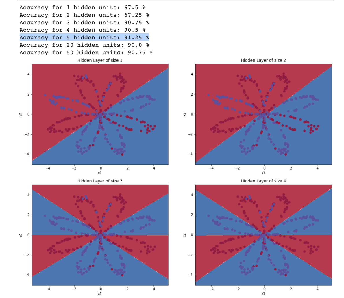
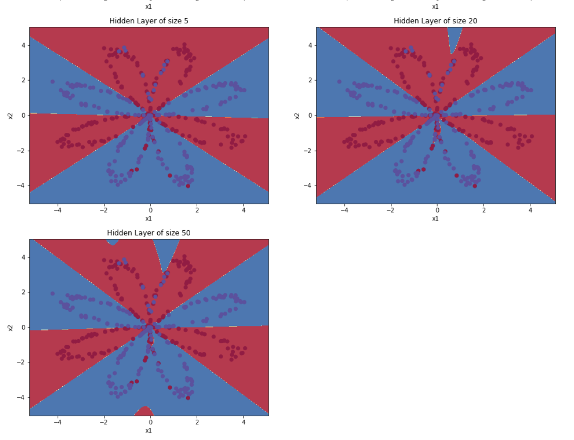
plt.figure(figsize=(16, 32))
hidden_layer_sizes = [1, 2, 3, 4, 5, 20, 50]
for i, n_h in enumerate(hidden_layer_sizes):
    plt.subplot(5, 2, i+1)
    plt.title('Hidden Layer of size %d' % n_h)
    parameters = nn_model(X, Y, n_h,1.2, num_iterations = 5000)
    plot_decision_boundary(lambda x: predict(parameters, x.T), X, Y)
    predictions = predict(parameters, X)
    accuracy = float((np.dot(Y,predictions.T) + np.dot(1-Y,1-predictions.T))/float(Y.size)*100)
    print ("Accuracy for {} hidden units: {} %".format(n_h, accuracy))

Output:

Interpretation:

The larger models (with more hidden units) are able to fit the training set better, until eventually the largest models overfit the data.
The best hidden layer size seems to be around n_h = 5. Indeed, a value around here seems to fits the data well without also incurring noticeable overfitting.