Statistical Learning Notes | Decision Tree 2 - Bagging & Random Forrest & Boosting

2020-11-17 1068 words 6 minutes

Contents

1.Bagging
– Out-of-Bag (OOB) Error Estimation
– Variable Importance Measures
2.Random Forest
– Decorrelating the Trees
3.boosting
– Algorithm
– Three Tuning Parameters

These three ensemble methods use trees as building blocks to construct more powerful prediction models

1. Bagging

Bootstrap is used when it is hard or even impossible to directly compute the Standard Deviation.

Bootstrap Aggregation (or bagging) can reduce the high-variance of decision trees

high variance may result in fitting quite different trees on different part of same data

A set of ${X_1,…,X_n}\ $ with variance $\sigma^2$
Averaging a set of observations $\bar{X}\ $ reduces variance to $\sigma^2/n \ $

To reduce the variance of a model and improve the prediction accuracy

Using B separate training sets from the population (hard since data may not enough)
Fit separate model $\hat{f}^1(x),…,\hat{f}^B(x)$
Average them to obtain a low-variance model:

$\hat{f}{avg} (x)= \frac{1}{B} \sum{b=1}^B \hat{f}^b(x)$

Bagging(Bootstrap) takes repeated samples from single trainging data set

Generate B different bootstrapped training data sets
then train the model on $b^{th}$ bootstrapped training set to get $\hat{f}^{*b}(x)$
Average all the predictions:

$$\hat{f}{bag}(x)=\frac{1}{B}\sum{b=1}^B\hat{f}^{*b}(x)$$

Bagging for Regression Tree:
Construct B regression trees using B bootstrapped training sets, these trees are grown deep and unpruned

each individual tree has high variance and low bias
Average these B trees to reduce the variance and improve accuracy

Bagging for Classification Tree:
Record the class predicted by each of the B trees, and take a majority vote:

The overall prediction is the most commonly occuring class among the B predictions.

Heart Disease Example:

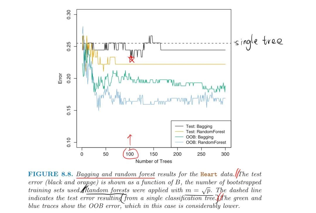
The number of trees B is not a critical parameter with bagging, large B will not lead to overfitting.

Out-of-Bag (OOB) Error Estimation

On average, each bagged tree makes use of around two-thirds of the observations,

the remaining one-third of the observations not used to fit a given bagged tree are referred to as the out-of-bag (OOB) observations

For the $i,^{th}$ observation, there will be around B/3 predictions to average or take a majority vote.

The resulting OOB error is a valid estimate of the test error for the bagged model

since the response for each observation is predicted using ONLY the trees that were NOT fit using that obseration

OOB replaces CV:
The OOB approach for estimating the Test Error is better when performing bagging on large data sets for which CV would be computationally onerous

as B sufficiently large, OOB error is virtually equivalent to LOOCV error

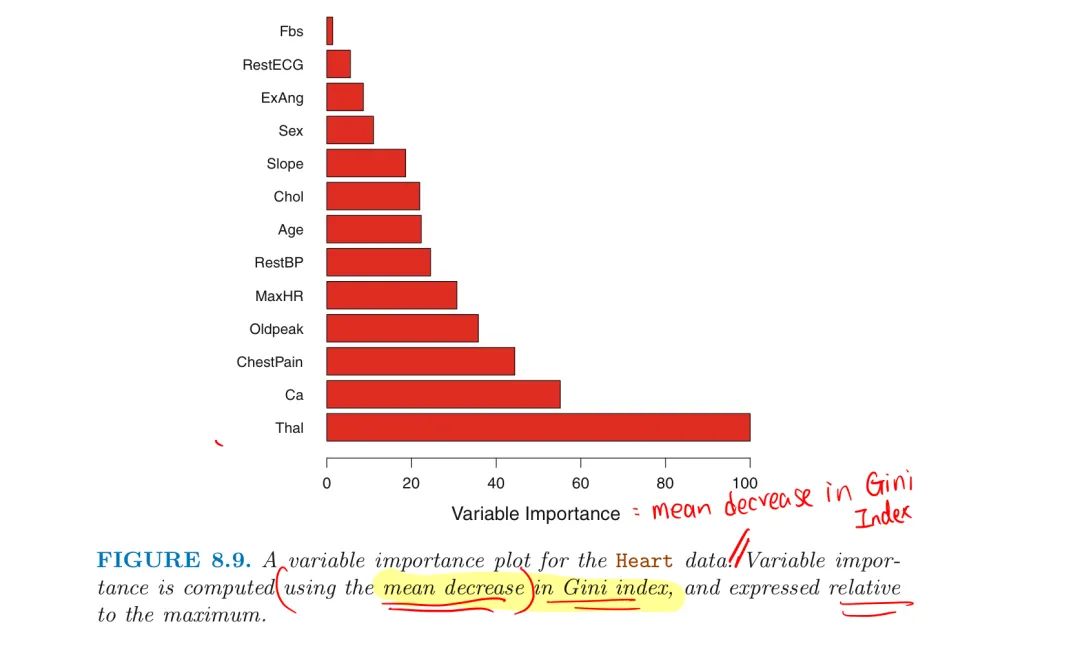
Variable Importance Measures

Bagging improves accuracy at the expense of interpretability

not clear which variables are important

Still can obtain an overall summary of the importance of each predictor by

Record the total amount that the RSS is decreased due to splits over given predictor for bagging regression trees
Add up the total amount that the Gini Index is decreased due to splits over given predictor for bagging classification trees
Average over all B trees and a large value indicates an important predictor

2. Random Forest

Random Forests provide an improvement over bagged trees by a way of a small tweak that decorrlates the trees.

As in bagging, RF builds a number of trees on bootstrapped training samples,

a random sample of m predictors is chosen as split candidates from all p predictors
a fresh resample of m predictors at each split and use ONE of those m predictors
$m\approx\sqrt{p}$

RF vs Bagging

The prediction from the bagged trees is highly correlated,

since most trees will use the strongest predictor in the top split
all of the bagged trees look quite similar

Decorrelating the Trees

RFs force each split to consider ONLY a subset of the predictors

on average (p-m)/p of the splits will NOT consider the strongest predictor
other predictors will have more of a chance to be considered at first
this makes the average of the resulting trees less variable and more reliable
and reduction in test error and OOB error

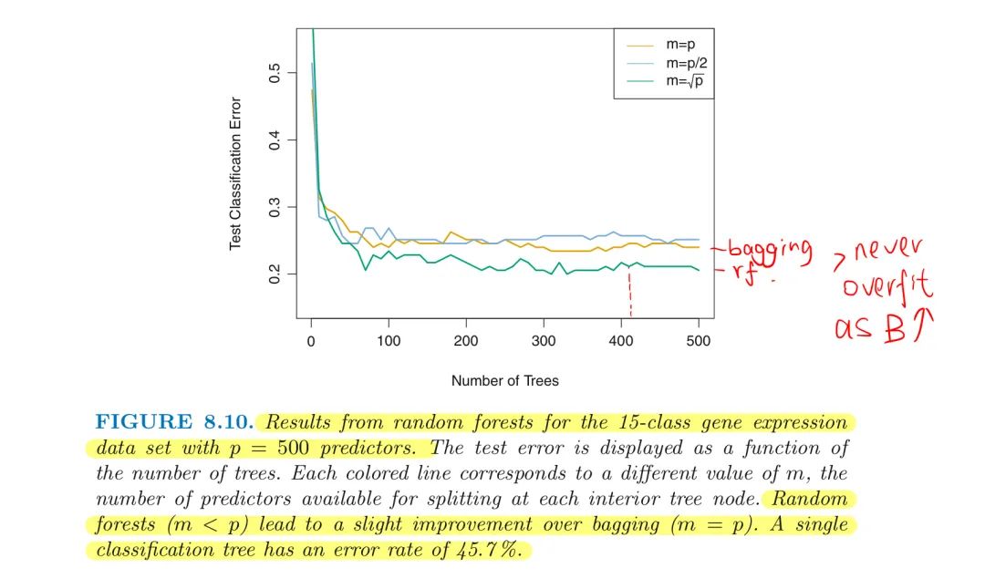
Small m will be helpful if a large number of correlated predictors

Example: RF on high-dimensional biology data includes 500 genes that have the largest variance in the training set

3. Boosting

Boosting does not involve bootstrap sampling

instead each tree is grown sequentially using information from previously grown trees
on a modified version of the original data set

Boosting for Regression Trees:

Set $\hat{f}(x)=0\ $ and $r_i=y_i \ $ for all i in the training set.
For b = 1,2,…,B, repeat:
(a) Fit a tree $\hat{f}^b$ with d splits (d+1 leaves) to the training data (X,r)
(b) Update $\hat{f}\ $ by adding in a shrunken version of the new tree: $$\hat{f}(x) \leftarrow \hat{f}(x)+\lambda\hat{f}^b(x)$$ (c) Update the Residuals: $$r_i \leftarrow r_i - \lambda\hat{f}^b(x_i)$$
Output the Boosted Model: $$\hat{f}(x)=\sum_{b=1}^B\lambda\hat{f}^b(x)$$

Explanation:

Fit a tree using the current residuals rather than Y

then add this new tree into the fitted function to update the residuals

Splits Parameter d controls each tree to be small with a few leaves

by fitting small trees to the residuals, we slowly improve $\hat{f}$
in areas where it does NOT perform well

The shrinkage parameter $\lambda\ $ slows the process down even further

allows more and different trees to attack the residuals

Idea:

The Boosting learns slowly

Unlike fitting a single large decision tree to the data, which amounts to fitting the data hard and potentially overfitting
Unlike in bagging, the construction of each tree depends strongly on the trees that have already been grown
In general, Statistical Learning methods that learn slowly tend to perform well

Three Tuning Parameters:

1.The number of trees B.

Large B leads to overfit for boosting, unlike bagging and RFs
Use CV to select B

2.The shrinkage parameter $\lambda$
$\lambda$ = 0.01 or 0.01 typically controls the boosting learning rate
a very small $\lambda\ $ can require using a very large B to perform well

3.The number d of splits in each tree
controls the complexity of the boosted ensemble
$d=1$ works well, in which case each tree is stump with single split
the boosted ensemble is fitting an additive model, since each term involves ONLY a single variable
d is the interaction depth that controls the interaction order of the boosted model, since d splits can involve at most d variables

Boosting vs RF

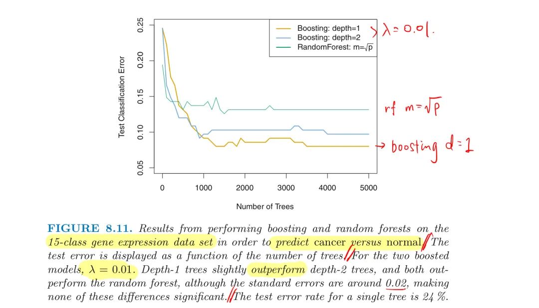
In boosting, since the growth of a particular tree takes into account the other trees that have already been grown, smaller trees are typically sufficient

using smaller trees can aid in interpretability
e.g. using stumps leads to an additive model