Decision Tree 1 - Regression and Classification Trees

0. Tree-based methods

Involving stratifying / segmenting the predictor space into a number of simple regions

• Use the mean/mode of the training data in the region as prediction for test data

1. Regression Decision Tree

1.1 Motivation

Making Prediction via Stratification of the Feature Space：

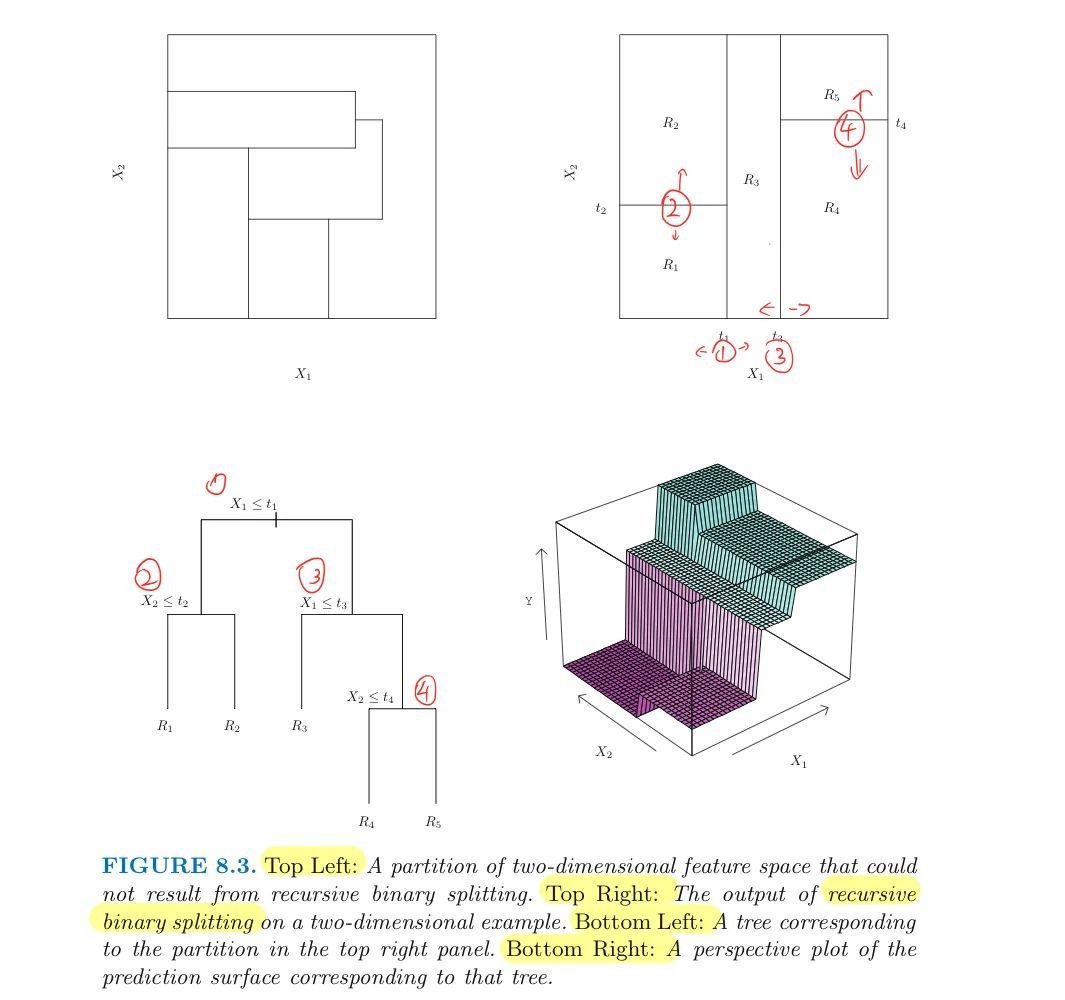
1. Divide the predictor space – that is, the set of possible response $Y$ for ${X_1,X_2,…,X_p}$ – into $J$ distinct and non-overlapping regions, ${R_1,R_2,…,R_J}$
2. For every test data which will fall into the region $R_j$, we make the same prediction, which is simply the mean of the response $Y$ for the training observations in $R_j$

1.2 Tree Splitting

The goal is to find leaves $R_1,…,R_J$ that minimizes the RSS, given by: $$\sum_{j=1}^J\sum_{i\in R_j}(y_i-\hat{y}_{R_j})^2$$

• where $\hat{y}_{R_j}$ is the mean response for the training observations within the $j,^{th}$ leaf

Problem: it is computationally infeasible to consider every possible partition of the feature space into $J$ leaves

Solution: Recursive Binary Splitting is a top-down, greedy approach:

• top-down because it begins at the top of the tree (all in one region) and then successively splits the predictor space;
• greedy because the best split is made at each step, rather than looking ahead globally and picking a split will lead to a better tree in some future step (which is impossible)

First, for any feature $p$ and cutpoint $s$ , we define two regions: $$R_1(p,s)={X|X_j< s}$$ $$and$$ $$R_2(p,s)={X|X_j\geq s}$$ to get the best $p$ and $s$ that minimize: $$\sum_{i:x_i\in R_1(p,s)}(y_i-\hat{y}_{R_1})^2+\sum_{i:x_i\in R_2(p,s)}(y_i-\hat{y}_{R_2})^2$$

Next, repeat the process, looking for the best $p$ and $s$ to continue splitting

• until a stopping criterion is reached:
• e.g. no region contains more than 5 observations.

If the number of features $p$ is not too large, this process can be done quickly

• predict $Y$ in test data using the mean of the train data in the region $R_j$ to which the test data belongs

1.3 Tree Pruning

Problem：Complex Tree will lead overfit (each leaf has one data)

Solution: A smaller tree with fewer splits (fewer $R_j\ $) may lead to lower variance and better interpretation at the cost of a little bias

Method 1 - Threshold
Splitting only as the decrease in the RSS exceeds some (high) threshold

• Problem: too short-sighted since a seemingly worthless split early on may lead to a better split with large reduction in RSS

Method 2 - Pruning
Grow a very large tree $T_0\ $, then prune it back in order to obtain a subtree

• Goal: select a subtree that leads to the lowest test error rate

Rather than CVing every possible subtree, we consider a sequence of trees indexed by non-negative tuning parameter $\alpha$

• Cost Complexity / Weakest Link Pruning

For each value of $\alpha$ there corresponds a subtree $T\subset T_0$ to minimize: $$\sum_{j=1}^{|T|}\sum_{i: \ x_i\in R_j}(y_i-\hat{y}_{Rj})^2 + \alpha|T|$$

• $|T|$ : number of leaves of the tree $T$

The tuning parameter $\alpha$ controls a trade-off between the subtree’s complexity and its fit to the training data.

• $\alpha= 0 => T = T_0$, just measures the error
• As $\alpha,$ increases, there is penalty for the subtree with many leaves
• so branches get pruned from the tree in a nested and predictable fashion,
• then obtaining the whole sequence of subtrees (as a function of $\alpha$ ) is easy

$\alpha$ is similar to $\lambda$ of the lasso, which is a controller of the complexity of a linear model

• also can be selected via CV and obtain the subtree corresponding to $\alpha$

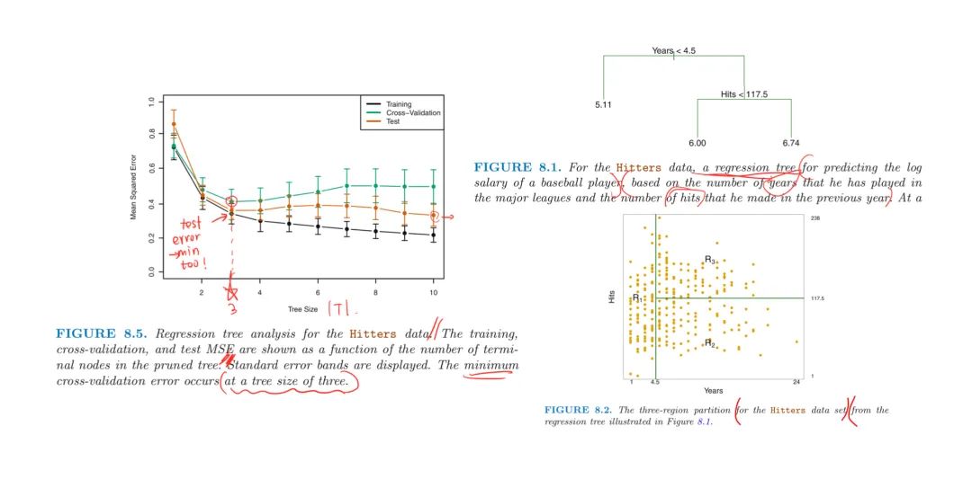
Example on Baseball Hitters Data

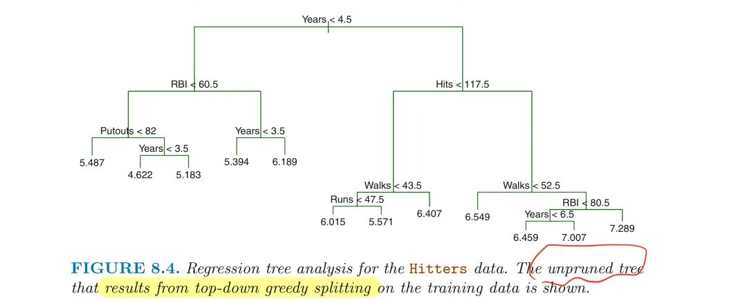
Perform 6-fold CV to estimate the CV MSE of the trees as a function of $\alpha$

• CV error is minimum at $|T|=3$ based on the best $\alpha$

2. Classification Trees

For a classification tree, we predict the test data belongs to the most commonly occurring class of train data in the region to which it belongs

• RSS cannot be a criterion for classification tree
• need two criterions to evaluate the quality of a particular split

Gini Index:
A measure of total variance across the $K$ classes: $$G=\sum_{k=1}^K\hat{p}_{mk}(1-\hat{p}_{mk})$$

• $\hat{p}_{mk}$ represents the proportion of train data in the $m^{th}$ region that are from the $k^{th}$ class
• G small if all $\hat{p}_{mk}$ are close 1 or 0
• Node Purity: Smaller if a node contains larger amount of observations from a single class

Cross-Entropy: $$D=-\sum_{k=1}^K\hat{p}_{mk}\log (\hat{p}_{mk})$$

• Like the Gini Index, the Entropy is smaller if $m^{th}$ node is pure
• both are sensitive to node purity

Heart Disease Example:

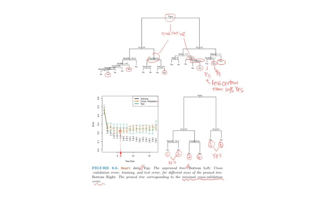
The splits may yield two same predicted value, there are reasons to keep them:

• because it leads to increased node purity
• improves the Gini Index and the Entropy

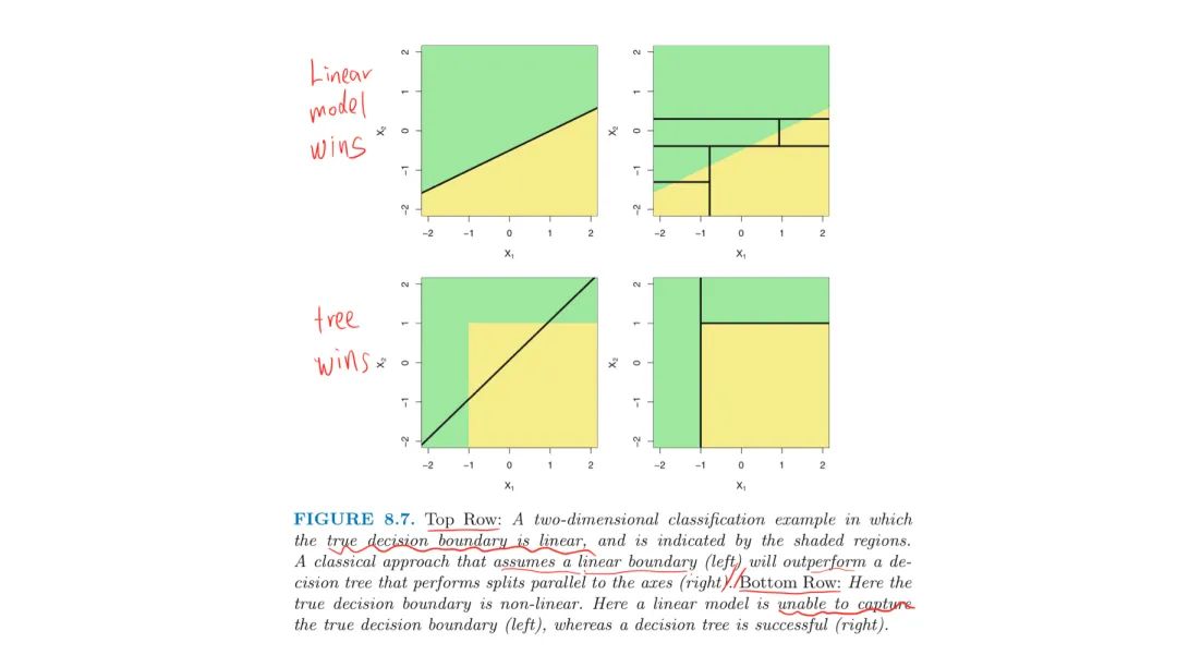
3. Trees vs Linear Models

If there is a highly non-linear complex relathinship between the features and the response, CARTs may outperform classical approaches

• However, there may still be linear relationship

4. Pros & Cons of Trees

Advantages:

1. Easier to interpret than Linear Regression
2. More closely mirror human decision making
3. Trees can be displayed graphically
4. Easily handle qualitative predictor without the dummy variables

Limitations:

1. Trees can be very non-robust:

• a small change in the data can cause a large change in the final estimated tree

2. Trees do not have the same level of predictive accuracy as other regression and classification methods

• TOGO：By aggregating many decision trees, bagging, random forests and boosting will improve accuracy, at the expense of some loss in interpretation

5. Reference

An Introduction to Statistical Learning, with applications in R (Springer, 2013)