Deep Learning Notes | Transfer Learning with MobileNets

2022-02-28 1805 words 9 minutes

Contents

Transfer Learning with MobileNets

Many machine learning methods work well ONLY under a common assumption: the training and test data are drawn from the same feature space and the same distribution.

When the distribution changes, most statistical models need to be rebuilt from scratch using newly collected training data.
In many realworld applications, it is expensive or impossible.
In such cases, Transfer Learning between task domains would be desirable.

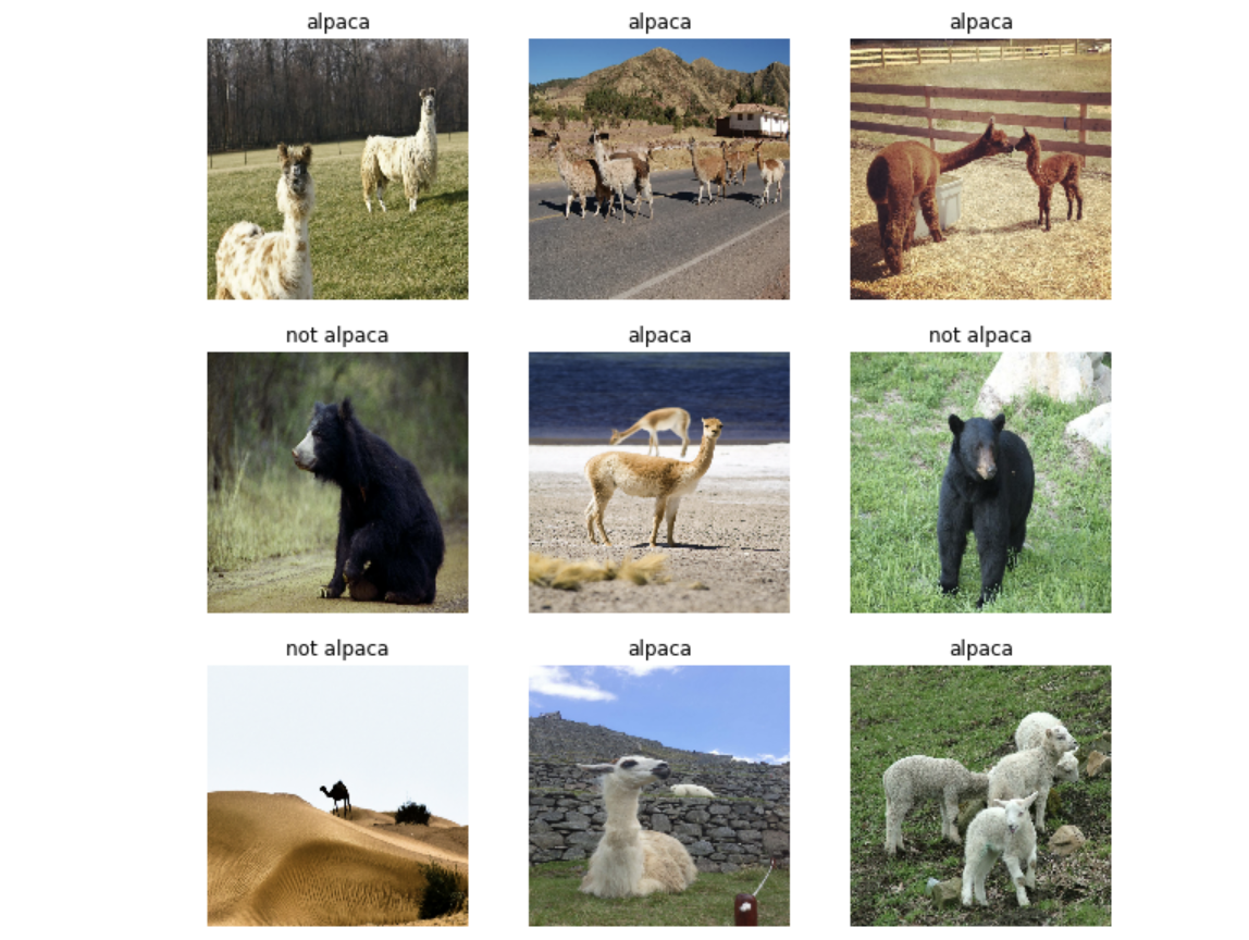
This note illustrate steps of using transfer learning on a pre-trained CNN to build an Alpaca/Not Alpaca （羊驼识别） classifier!

A pre-trained model is a network that’s already been trained on a large dataset and saved, which allows us to reuse the weights to customize our own model cheaply and efficiently.
The one we’ll be using, MobileNetV2, was designed to provide fast and computationally efficient performance
- at deployment for mobile and embedded applications
It’s been pre-trained on ImageNet, a dataset containing over 14 million images and 1000 classes.

1. Create and Split the Dataset

 1
 2
 3
 4
 5
 6
 7
 8
 9
10
11
12
13
14
15
16
17
18
19
20
21
22
23
24
25
26
27


import matplotlib.pyplot as plt
import numpy as np
import os
import tensorflow as tf
import tensorflow.keras.layers as tfl

from tensorflow.keras.preprocessing import image_dataset_from_directory
from tensorflow.keras.layers.experimental.preprocessing import RandomFlip, RandomRotation

BATCH_SIZE = 32
IMG_SIZE = (160, 160)
directory = "dataset/"
train_dataset = image_dataset_from_directory(directory,
                                             shuffle=True,
                                             batch_size=BATCH_SIZE,
                                             image_size=IMG_SIZE,
                                             validation_split=0.2,
                                             subset='training',
                                             seed=42)

validation_dataset = image_dataset_from_directory(directory,
                                             shuffle=True,
                                             batch_size=BATCH_SIZE,
                                             image_size=IMG_SIZE,
                                             validation_split=0.2,
                                             subset='validation',
                                             seed=42)

Found 327 files belonging to 2 classes.
Using 262 files for training.
Found 327 files belonging to 2 classes.
Using 65 files for validation.

Visualize the Images

1
2
3
4
5
6
7
8
9


class_names = train_dataset.class_names

plt.figure(figsize=(10, 10))
for images, labels in train_dataset.take(1):
    for i in range(9):
        ax = plt.subplot(3, 3, i + 1)
        plt.imshow(images[i].numpy().astype("uint8"))
        plt.title(class_names[labels[i]])
        plt.axis("off")

2. Preprocess and Augment Training Data

Using prefetch() prevents a memory bottleneck that can occur when reading from disk. It sets aside some data and keeps it ready for when it’s needed, by creating a source dataset from input data, applying a transformation to preprocess it, then iterating over the dataset one element at a time.

Because the iteration is streaming, the data doesn’t need to fit into memory.

Use tf.data.experimental.AUTOTUNE to choose the parameters automatically. Autotune prompts tf.data to tune that value dynamically at runtime, by tracking the time spent in each operation and feeding those times into an optimization algorithm.

The optimization algorithm tries to find the best allocation of its CPU budget across all tunable operations.

1
2


AUTOTUNE = tf.data.experimental.AUTOTUNE
train_dataset = train_dataset.prefetch(buffer_size=AUTOTUNE)

To increase diversity in the training set and help the model learn the data better,

it’s standard practice to augment the images by transforming them
- i.e., randomly flipping and rotating them.
Keras' Sequential API offers a straightforward method for these kinds of data augmentations, with built-in, customizable preprocessing layers.
These layers are saved with the rest of your model and can be re-used later.

 1
 2
 3
 4
 5
 6
 7
 8
 9
10
11
12
13
14
15
16
17
18
19
20
21
22


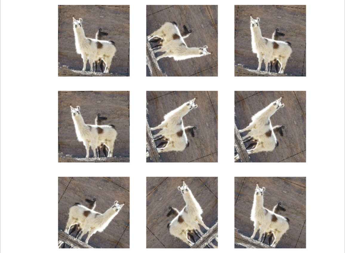
def data_augmenter():
    '''
    Create a Sequential model composed of 2 layers
    Returns:
        tf.keras.Sequential
    '''
    data_augmentation = tf.keras.Sequential()
    data_augmentation.add(RandomFlip('horizontal'))
    data_augmentation.add(RandomRotation(0.2))

    return data_augmentation
####################################
data_augmentation = data_augmenter()

for image, _ in train_dataset.take(1):
    plt.figure(figsize=(10, 10))
    first_image = image[0]
    for i in range(9):
        ax = plt.subplot(3, 3, i + 1)
        augmented_image = data_augmentation(tf.expand_dims(first_image, 0))
        plt.imshow(augmented_image[0] / 255)
        plt.axis('off')

3. Using MobileNetV2 for Transfer Learning

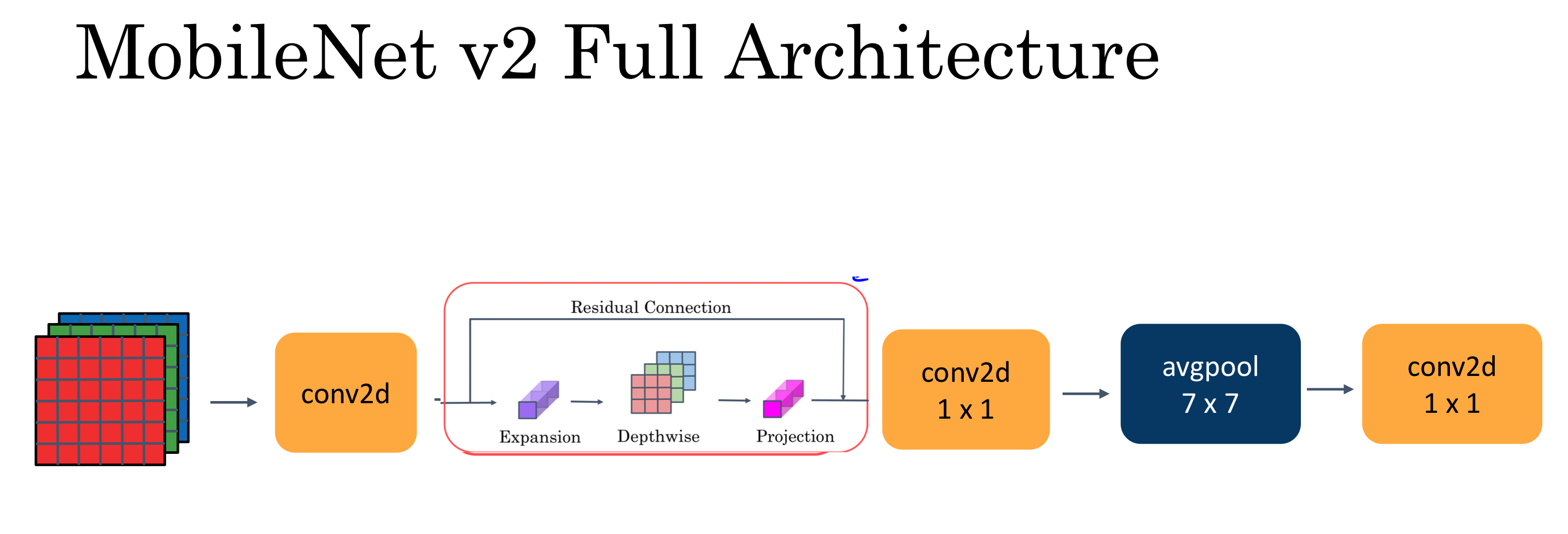
MobileNetV2 was trained on ImageNet and is optimized to run on mobile and other low-power applications.

It’s 155 layers deep and very efficient for object detection and image segmentation tasks, as well as classification tasks like this one.

The architecture has three defining characteristics:

Depthwise separable convolutions
- to reduce the number of trainable parameters and operations
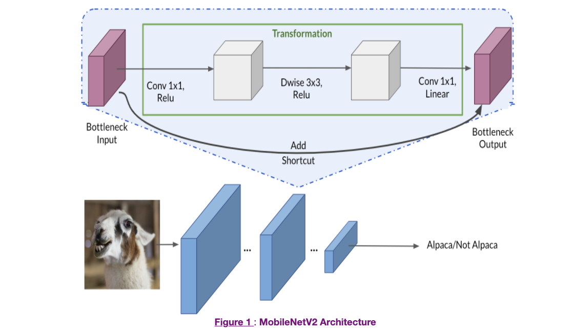
Thin input and output bottlenecks between layers
- these bottlenecks encode the intermediate inputs and outputs in a low dimensional space,
- and prevent non-linearities from destroying important information.
Shortcut connections between bottleneck layers
- to speed up training and improving predictions.

Speed up convolutions in two steps

Depthwise Convolution calculates an intermediate result

by convolving on each of the channels independently.
it provides lightweight feature filtering and creation
deal with both spatial and depth (number of channels) dimensions

Pointwise Convolution merges the outputs of the previous step into one.

This gets a single result from a single feature at a time,
and then is applied to all the filters in the output layer.

1
2
3
4
5
6
7
8


preprocess_input = tf.keras.applications.mobilenet_v2.preprocess_input

IMG_SHAPE = IMG_SIZE + (3,)
base_model = tf.keras.applications.MobileNetV2(input_shape=IMG_SHAPE,
                                               include_top=True,
                                               weights='imagenet')

base_model.summary()

Check Batch

The number 32 refers to the batch size and 1000 refers to the 1000 classes the model was pretrained on.

 1
 2
 3
 4
 5
 6
 7
 8
 9
10


image_batch, label_batch = next(iter(train_dataset))
feature_batch = base_model(image_batch)
print(feature_batch.shape) # (32, 1000)

#Shows the different label probabilities in one tensor
label_batch
'''
<tf.Tensor: shape=(32,), dtype=int32, numpy=
array([1, 0, 0, 1, 1, 1, 0, 1, 1, 1, 0, 0, 0, 1, 1, 1, 1, 1, 1, 0, 1, 0, 0, 0, 1, 0, 1, 1, 1, 1, 0, 0], dtype=int32)>
'''

Predictions

The predictions returned by the base model below follow this format:

First the class number, then a human-readable label, and last the probability of the image belonging to that class.
there are two of these returned for each image in the batch - these the top two probabilities returned for that image.

1
2
3
4
5


base_model.trainable = False
image_var = tf.Variable(image_batch)
pred = base_model(image_var)

tf.keras.applications.mobilenet_v2.decode_predictions(pred.numpy(), top=2)

Because MobileNet pretrained over ImageNet doesn’t have the correct labels for alpacas, so using the full model will get a bunch of incorrectly classified images.

Solution: delete the top layer, which contains all the classification labels, and create a new classification layer.

4. Modify Pretrained Model by Layer Freezing

To use a pretrained model to modify the classifier task so that it’s able to recognize alpacas, we need:

Delete the top layer (the classification layer)
- include_top=False
Add a new trained classifier layer by freezing the rest of the network
- a single neuron is enough to solve a binary classification problem.
Freeze the base model and train the newly-created classifier layer
- base_model.trainable=False
- base_model(x, training=False)

 1
 2
 3
 4
 5
 6
 7
 8
 9
10
11
12
13
14
15
16
17
18
19
20
21
22
23
24
25
26
27
28
29
30
31
32
33
34
35
36
37
38
39
40
41
42
43
44
45
46
47
48
49
50
51
52
53


def alpaca_model(image_shape=IMG_SIZE, data_augmentation=data_augmenter()):
    ''' Define a tf.keras model for binary classification out of the MobileNetV2 model
    Arguments:
        image_shape -- Image width and height
        data_augmentation -- data augmentation function
    Returns:
    Returns:
        tf.keras.model
    '''
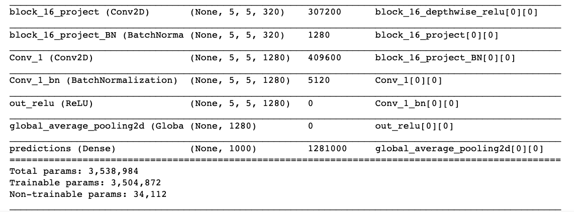
    input_shape = image_shape + (3,)

    base_model = tf.keras.applications.MobileNetV2(
        input_shape=input_shape,
        include_top=False, # <== Important!!!!
        weights='imagenet') # From imageNet

    # Freeze the base model by making it non trainable
    base_model.trainable = False
    # Create the input layer (Same as the imageNetv2 input size)
    inputs = tf.keras.Input(shape=input_shape)
    # Apply data augmentation to the inputs
    x = data_augmentation(inputs)
    # Data preprocessing using the same weights the model was trained on
    x = preprocess_input(x)
    # Set training to False to avoid keeping track of statistics in the batch norm layer
    x = base_model(x, training=False)
    # Add the new Binary classification layers
    # Use global avg pooling to summarize the info in each channel
    x = tfl.GlobalAveragePooling2D()(x)
    # Include dropout with probability of 0.2 to avoid overfitting
    x = tfl.Dropout(0.2)(x)

    # Use a prediction layer with one neuron (as a binary classifier only needs one)
    outputs = tfl.Dense(1)(x)

    model = tf.keras.Model(inputs, outputs)

    return model

model2 = alpaca_model(IMG_SIZE, data_augmentation)
for layer in summary(model2):
    print(layer)
'''
['InputLayer', [(None, 160, 160, 3)], 0]
['Sequential', (None, 160, 160, 3), 0]
['TensorFlowOpLayer', [(None, 160, 160, 3)], 0]
['TensorFlowOpLayer', [(None, 160, 160, 3)], 0]
['Functional', (None, 5, 5, 1280), 2257984]
['GlobalAveragePooling2D', (None, 1280), 0]
['Dropout', (None, 1280), 0, 0.2]
['Dense', (None, 1), 1281, 'linear']
'''

Model Compile and Visualize Accuracy

 1
 2
 3
 4
 5
 6
 7
 8
 9
10
11
12
13
14
15
16
17
18
19
20
21
22
23
24
25
26
27
28
29
30
31
32


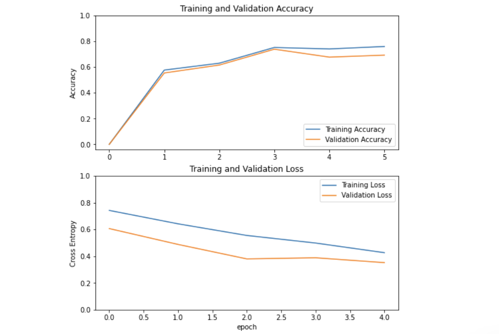
base_learning_rate = 0.001
model2.compile(optimizer=tf.keras.optimizers.Adam(lr=base_learning_rate),
              loss=tf.keras.losses.BinaryCrossentropy(from_logits=True),
              metrics=['accuracy'])

initial_epochs = 5
history = model2.fit(train_dataset, validation_data=validation_dataset, epochs=initial_epochs)

acc = [0.] + history.history['accuracy']
val_acc = [0.] + history.history['val_accuracy']

loss = history.history['loss']
val_loss = history.history['val_loss']

plt.figure(figsize=(8, 8))
plt.subplot(2, 1, 1)
plt.plot(acc, label='Training Accuracy')
plt.plot(val_acc, label='Validation Accuracy')
plt.legend(loc='lower right')
plt.ylabel('Accuracy')
plt.ylim([min(plt.ylim()),1])
plt.title('Training and Validation Accuracy')

plt.subplot(2, 1, 2)
plt.plot(loss, label='Training Loss')
plt.plot(val_loss, label='Validation Loss')
plt.legend(loc='upper right')
plt.ylabel('Cross Entropy')
plt.ylim([0,1.0])
plt.title('Training and Validation Loss')
plt.xlabel('epoch')
plt.show()

Right Now, the modified model has learned the class_names for given training dataset

['alpaca', 'not alpaca']

5. Fine-tuning the Final Layers

Fine-tuning the model by re-running the optimizer in the last layers can improve accuracy.

a smaller learning rate takes smaller steps to adapt it a little more closely to the new data.

In Transfer Learning, unfreezing the layers at the end of the network, and then re-training your model on the final layers with a very low learning rate.

the low-level features can be kept the same, as they have common features for most images.
we want the high-level features adapt to new data, which is rather like letting the network learn to detect features more related to new training data, such as soft fur or big teeth.
the later layers are the part of the network that contain the fine details (pointy ears, hairy tails) that are more specific to problem.

 1
 2
 3
 4
 5
 6
 7
 8
 9
10
11
12
13
14
15
16
17
18
19
20
21
22
23
24
25
26
27
28
29
30
31
32


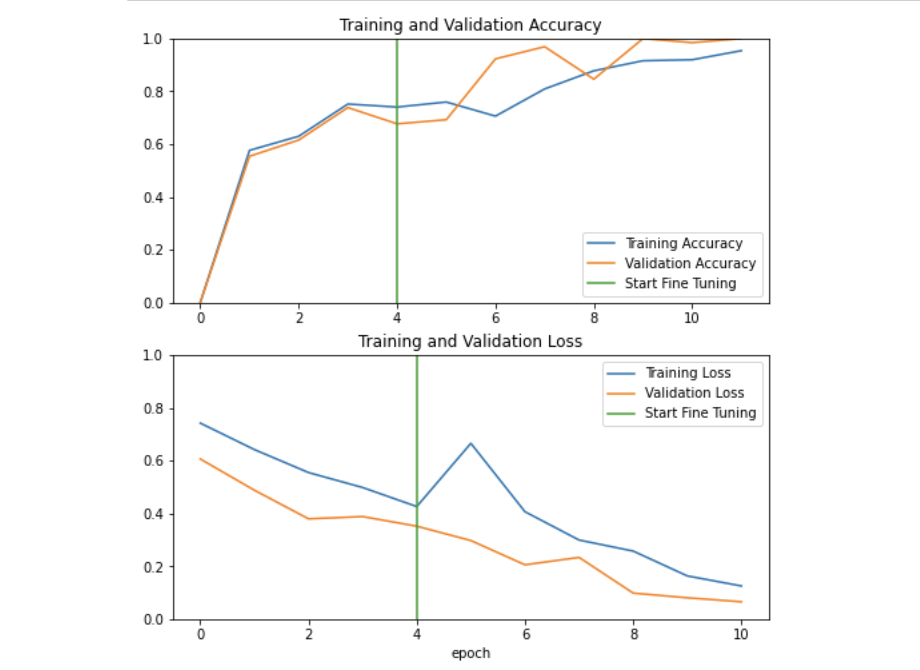
base_model = model2.layers[4]
base_model.trainable = True

# 155 layers are in the base model
print("Number of layers in the base model: ", len(base_model.layers))

# Fine-tune from this layer onwards
fine_tune_at = 120

# Freeze all the layers before the `fine_tune_at` layer
for layer in base_model.layers[:fine_tune_at]:
    layer.trainable = None

# Define a BinaryCrossentropy loss function. Use from_logits=True
loss_function=tf.keras.losses.BinaryCrossentropy(from_logits=True)
# Define an Adam optimizer with a learning rate of 0.1 * base_learning_rate
optimizer = tf.keras.optimizers.Adam(learning_rate=base_learning_rate*0.1)
# Use accuracy as evaluation metric
metrics=['accuracy']


model2.compile(loss=loss_function,
              optimizer = optimizer,
              metrics=metrics)

fine_tune_epochs = 5
total_epochs =  initial_epochs + fine_tune_epochs

history_fine = model2.fit(train_dataset,
                         epochs=total_epochs,
                         initial_epoch=history.epoch[-1],
                         validation_data=validation_dataset)

Visualize Accuracy

 1
 2
 3
 4
 5
 6
 7
 8
 9
10
11
12
13
14
15
16
17
18
19
20
21
22
23
24
25
26


acc += history_fine.history['accuracy']
val_acc += history_fine.history['val_accuracy']

loss += history_fine.history['loss']
val_loss += history_fine.history['val_loss']

plt.figure(figsize=(8, 8))
plt.subplot(2, 1, 1)
plt.plot(acc, label='Training Accuracy')
plt.plot(val_acc, label='Validation Accuracy')
plt.ylim([0, 1])
plt.plot([initial_epochs-1,initial_epochs-1],
          plt.ylim(), label='Start Fine Tuning')
plt.legend(loc='lower right')
plt.title('Training and Validation Accuracy')

plt.subplot(2, 1, 2)
plt.plot(loss, label='Training Loss')
plt.plot(val_loss, label='Validation Loss')
plt.ylim([0, 1.0])
plt.plot([initial_epochs-1,initial_epochs-1],
         plt.ylim(), label='Start Fine Tuning')
plt.legend(loc='upper right')
plt.title('Training and Validation Loss')
plt.xlabel('epoch')
plt.show()