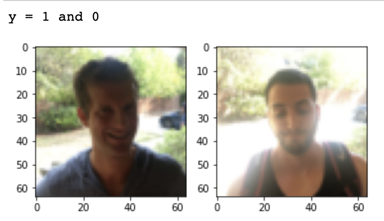
X_train_orig,Y_train_orig,X_test_orig,Y_test_orig,classes=load_happy_dataset()# Normalize image vectorsX_train=X_train_orig/255.X_test=X_test_orig/255.# ReshapeY_train=Y_train_orig.TY_test=Y_test_orig.T# Visualizef,axarr=plt.subplots(1,2)# use the created array to output your multiple images. In this case I have stacked 4 images verticallyaxarr[0].imshow(X_train_orig[9])axarr[1].imshow(X_train_orig[124])print("y = "+str(np.squeeze(Y_train_orig[:,9]))+" and "+str(np.squeeze(Y_train_orig[:,124])))
1.1. TF Keras Sequential API
This API allows us to build layer by layer with exactly one input tensor and one output tensor
Sequential layers are ordered, and the order in which they are specified matters.
If the model is non-linear or contains layers with multiple inputs or outputs, a Sequential model wouldn’t be the right choice!
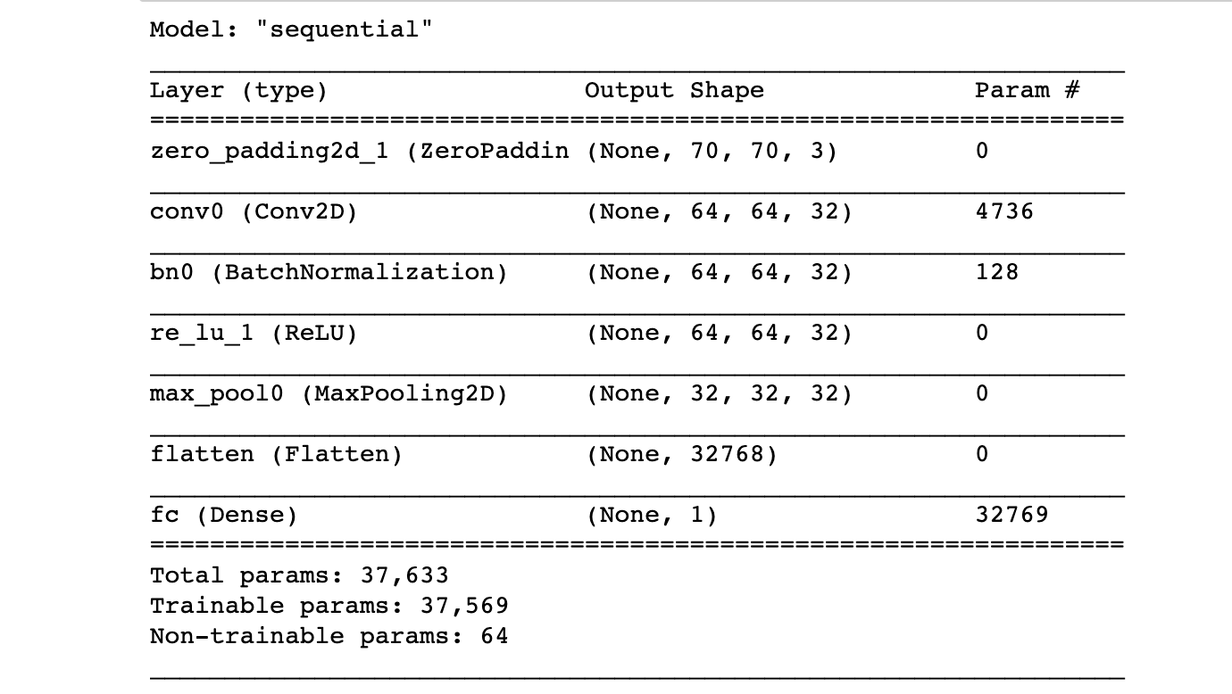
defhappyModel():"""
Implements the forward propagation for the binary classification model:
ZEROPAD2D -> CONV2D -> BATCHNORM -> RELU -> MAXPOOL -> FLATTEN -> DENSE
Note that for simplicity and grading purposes, you'll hard-code all the values
such as the stride and kernel (filter) sizes.
Normally, functions should take these values as function parameters.
Arguments:
None
Returns:
model -- TF Keras model (object containing the information for the entire training process)
"""model=tf.keras.Sequential([## 1. ZeroPadding2D with padding 3, input shape of 64 x 64 x 3tf.keras.layers.ZeroPadding2D(padding=(3,3),input_shape=(64,64,3),data_format="channels_last"),## 2. Conv2D with 32 7x7 filters and stride of 1tf.keras.layers.Conv2D(32,(7,7),strides=(1,1),name='conv0'),## 3. BatchNormalization for axis 3tf.keras.layers.BatchNormalization(axis=3,name='bn0'),## 4.ReLUtf.keras.layers.ReLU(max_value=None,negative_slope=0.0,threshold=0.0),## 5. Max Pooling 2D with default parameterstf.keras.layers.MaxPooling2D((2,2),name='max_pool0'),## 6. Flatten layertf.keras.layers.Flatten(),## 7. Dense layer with 1 unit for output & 'sigmoid' activationtf.keras.layers.Dense(1,activation='sigmoid',name='fc'),])returnmodel
Use .evaluate() to evaluate against the test set. This function will print the value of the loss function and the performance metrics specified during the compilation of the model.
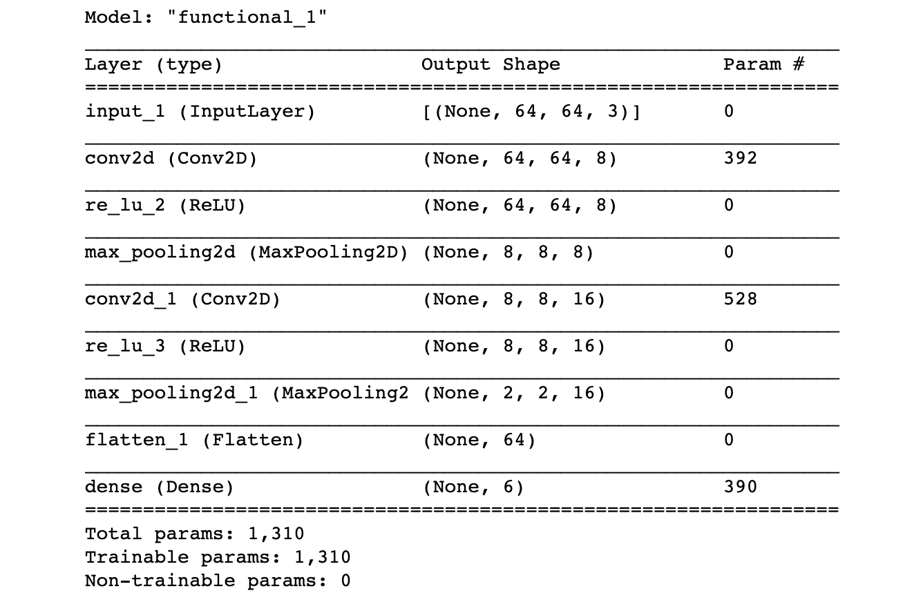
defconvolutional_model(input_shape):"""
Implements the forward propagation for the model:
CONV2D -> RELU -> MAXPOOL -> CONV2D -> RELU -> MAXPOOL -> FLATTEN -> DENSE
Note that for simplicity and grading purposes, you'll hard-code some values
such as the stride and kernel (filter) sizes.
Normally, functions should take these values as function parameters.
Arguments:
input_img -- input dataset, of shape (input_shape)
Returns:
model -- TF Keras model (object containing the information for the entire training process)
"""input_img=tf.keras.Input(shape=input_shape)## CONV2D: 8 filters 4x4, stride of 1, padding 'SAME'Z1=tf.keras.layers.Conv2D(filters=8,kernel_size=(4,4),strides=(1,1),padding='same')(input_img)## RELUA1=tf.keras.layers.ReLU()(Z1)## MAXPOOL: window 8x8, stride 8, padding 'SAME'P1=tf.keras.layers.MaxPool2D(pool_size=(8,8),strides=(8,8),padding='same')(A1)## CONV2D: 16 filters 2x2, stride 1, padding 'SAME'Z2=tf.keras.layers.Conv2D(filters=16,kernel_size=(2,2),strides=(1,1),padding='same')(P1)## RELUA2=tf.keras.layers.ReLU()(Z2)## MAXPOOL: window 4x4, stride 4, padding 'SAME'P2=tf.keras.layers.MaxPool2D(pool_size=(4,4),strides=(4,4),padding='same')(A2)## FLATTENF=tf.keras.layers.Flatten()(P2)## Dense layer:## Apply a fully connected layer with 6 neurons and a softmax activation.outputs=tf.keras.layers.Dense(units=6,activation='softmax')(F)model=tf.keras.Model(inputs=input_img,outputs=outputs)returnmodel
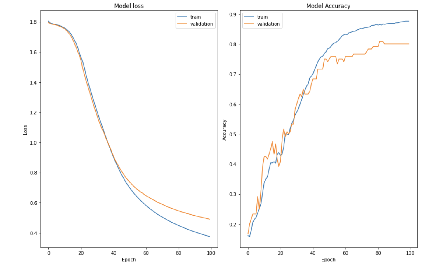
The history object is an output of the .fit() operation, and provides a record of all the loss and metric values in memory. It’s stored as a dictionary that you can retrieve at history.history: